Formulas Part 3: In full swing
Among the formula functions in RagTime, there are two in particular that can be used to create actual scripts: horizontal and vertical searches. When working with large data sets (such as addresses, etc.), it is virtually impossible to work efficiently without these functions. However, it is necessary to understand the logic behind how a search works. Let's get started (and RagTime too)!
The «VSearch» function does nothing more than search for something in a spreadsheet. It always searches within a defined range, row by row, to find cell contents that meet a specific condition.
In the simplest form of the function, it only counts how often the condition is met. During the search, a counter is kept track of that indicates how many rows have already been examined. If the range starts in row 1 of a spreadsheet, this counter indicates the number of the row that is currently being viewed.
The current counter value is returned by the «CurrentIndex» function (a function that can only be used within search functions). Not only the row, but also the cell currently being checked in the first column of the search range can be queried with a function: with «CurrentCell». For example:

This formula counts how often the name «Smith» appears in column A. The search works as follows: all cells in column A are examined, starting in row 1. The «CurrentIndex» is therefore = 1, and it is increased with each row examined. The value of the function itself is set to 0.
In each row of column A containing the name being searched for, the result of the function is increased by 1. However, this cannot be tracked because the function is calculated in one go. At the end, the function simply returns the desired number, i.e., the number of «Smith» in column A.
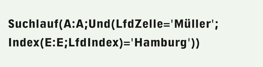
However, the condition in the function can also be more complicated. For example, if you want to know how many «Smith» are in the table who live in Hamburg, the formula is as follows, assuming the place of residence is in column E of the table:

«And» links the following conditions: all of them must be met for the row to be counted as a “hit”. This means that the term «Hamburg» must also appear in the fifth column. The function «ColumnValue(5)» queries the content of the row currently being examined in column E. However, we strongly advise against using the «ColumnValue» function in this form (with explicit specification of the column number)! If you later insert a column in the search area, e.g., for a country code before the column with the postal code, the search area would be adjusted to A:F, but the 5 as the argument of the column value function would not be adjusted – and the formula would fail.
Searching for errors in formulas that once worked perfectly and suddenly no longer deliver the expected result after a seemingly insignificant change to the document can be utterly frustrating. Instead, write:
The search range can remain limited to A:A in Formula F-3.3, as the index function, unlike «ColumnValue», can also refer to cells outside the search range specified in the function. And since only a single column is searched, the «Search» function is sufficient instead of «VSearch». The «Index» function addresses the cell in column E that is on the same row as the cell currently being examined in column A. This is ensured by using the current search counter, which is used for addressing with the «CurrentIndex» function. If a new column C is now inserted in the table, RagTime correctly adjusts the column reference in the index function for this formula syntax.
If the table contains a header row, this is irrelevant in this case, as it certainly does not contain «Smith/Toronto». In other cases, another condition would have to be added to the AND function:

Of course, the comparison value must be increased if the automatic table header contains more than one header row.
So far, we have described how the search function works. Now let's turn to the more complex forms of this function.
In many cases, we don't just want to count, we want a specific result based on the values in the “hit row”. A concrete example: a delivery note (in a spreadsheet) lists various items, but not all of them are in stock (see Fig. F-3.1).
For all items that are in stock, column F shows today's date as the delivery date. Column H shows the prices. For today's invoicing, we want to determine the total price of those items that are being delivered today. To do this, we need the search function as specified in the function list in its second form, i.e.:
Translated with DeepL.com (free version)

In our example, we are looking for all positions where today's date is contained in column F. Consequently, the first two arguments of the function are clear: the «Range» is F:F and the «Condition» is «CurrentCell=today».
The search function determines the «NextValue» for each hit. This is determined by a formula that can be specified here as the fourth argument. We want to add up the prices of all “hit rows.” To do this, we need a result from column H. The running total (after each search step) is specified by the «CurrentResult» function – another function that is only available in connection with search functions. Before processing the first row, «CurrentResult» takes the value specified by the «StartValue» argument and is replaced by the result of the formula for the «NextValue» after each “hit row” has been processed. So we set the «StartValue» to 0. The «NextValue» is calculated by adding «CurrentResult» and the value in column H. Formula F-3.6 is therefore the complete search run with all these arguments.
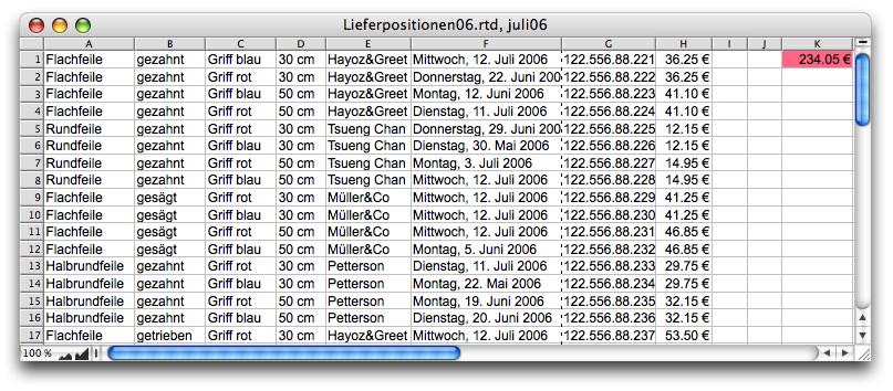
Once the search is complete, the result of the entire formula is equal to the last «NextValue» determined. The result is therefore displayed where the search function formula was entered. In our case, this is cell K1 (see Fig. F-3.1).

This euro amount can, of course, also appear in the middle of a continuous text if the formula has been entered there. However, we can also use the result in a second location – for example, in another spreadsheet – by combining the Formula F-3.6 with the «SetCell» function.
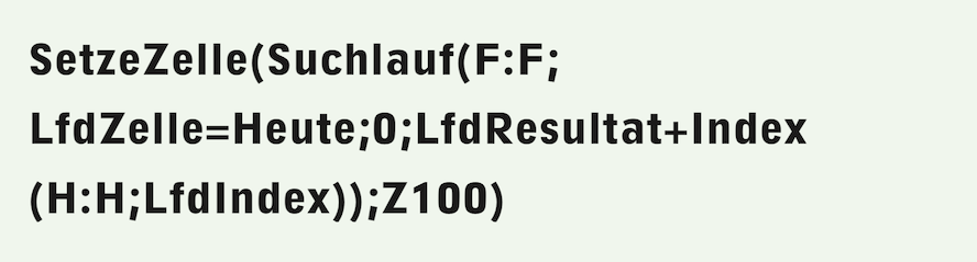
The «SetCell» function has several variants with different arguments in the function list. The first variant is sufficient for our purposes here. It writes a value to a cell with a fixed address, in this case cell Z100, according to Formula F-3.7.

At the same time, however, the value also appears where the formula itself was entered. It therefore places the text «Result of the search function» in cell Z100 and leaves the same text where the formula is located. Of course, we don't want this text, but rather the actual result of the search function. So, after «SetCell», we add our previous search formula, so that everything – once combined – results in the Formula F-3.8:
Just like buttons or recurring layout and corporate design elements, complex formulas must also be documented. Even experienced RagTime users quickly lose track of exactly what a formula they wrote themselves does, especially after several months. Then every attempt to understand the meaning of a formula and how it works becomes a guessing game.
Unfortunately, the individual functions in the RagTime formula palette cannot be structured or supplemented with comments. As is well known, formula entries must be strung together without spaces or line breaks. This makes them difficult to read and analyze.
The more complicated and nested a formula is, the more problematic it becomes. It is almost impossible to check. Only documentation can help here. Here we suggest a possible method, which we will then continue to use in the following. In a document with formulas, we create an additional spreadsheet called «DOK». However, you can also create your own document with several such DOK spreadsheets to create an archive of formulas.
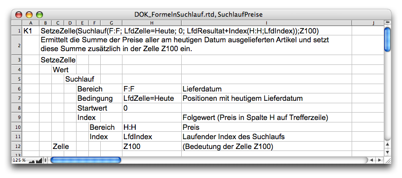
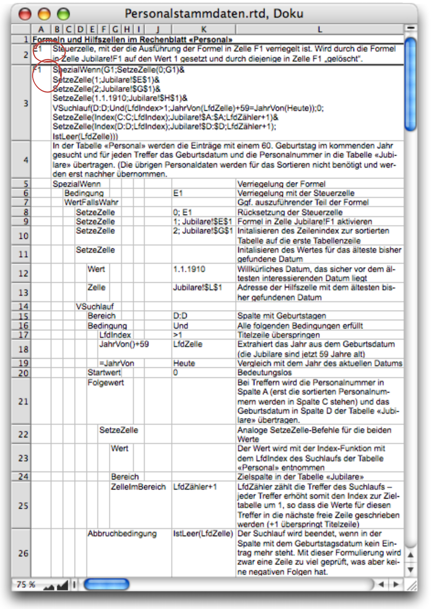
To ensure that you can nod your head or say “aha – yes, of course” every time, it is best to structure each complex formula according to functions and explanations, as shown in Fig. F-3.2. The first line contains the address of the cell containing the formula. Next to it is the complete formula, which you can copy from the formula palette. The field with the formula can also be formatted as a multi-line field, so that longer formulas can be presented more clearly with an outline. However, if you want to create a formula archive so that you can copy the formulas from here to the formula palette as needed, you must make sure to remove all line breaks and spaces.
A description of the formula's function follows immediately below the formula. It is advisable to make this as precise as possible and to relate it to the specific case of application.
Finally, each function used is explained with its arguments. Each nesting is made visible by corresponding indentation. For the outermost function («SetCell»), the two arguments are found in the next indentation level: first the function «Search», which determines the value to be inserted, then the addressing where this value is to be inserted. Similarly, the search function is “dissected” at the next level.
For better understanding, the syntactic definitions of the individual arguments are also listed here. This type of documentation may seem a little excessive. But you will soon realize how useful it is when dealing with really complicated formulas.
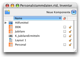
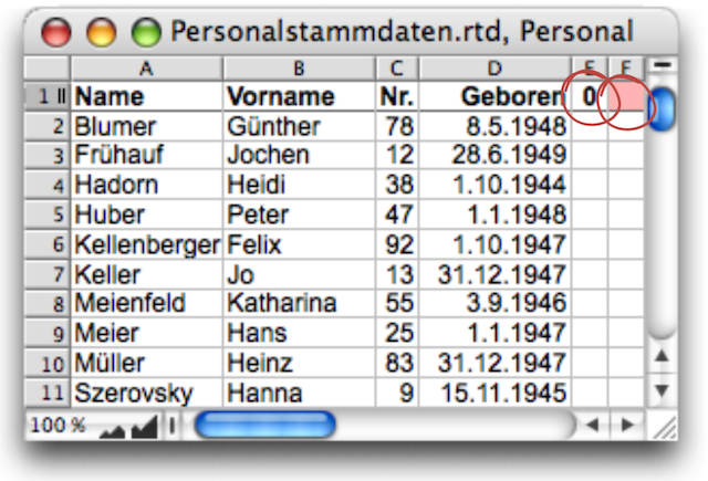
We would like to use another practical example to further illustrate the qualities of the search function: We have a document with a «Personnel» spreadsheet and an «Anniversaries» spreadsheet. From the «Personnel» spreadsheet – which contains data on employees – we want to extract those who will reach the age of 60 next year. This is a typical scenario that occurs repeatedly in a similar form for form letters, invitations, etc. It involves extracting and sorting according to changing or current criteria. We will go into more detail on the following page. Here, we have limited the personnel data to the minimum required for the example.
Before we tackle the solution, two concepts for applying complex formulas in spreadsheets are helpful: breaking formulas down into subformulas that are made dependent on each other, on the one hand, and using headers for formulas, auxiliary cells, and buttons, on the other.
Breaking down complex formulas into subformulas has one important advantage: by decoupling the sub-steps – suppressing the triggering of the subsequent subformula – the entire calculation process can be tested in steps. In the chapter “Formulas Part 2: Variety of buttons”, we created a «Color Choice» button (And this becomes a button…). Each time a color selection button was pressed, a 1 was written to the control cell D2. This enabled the execution of a formula that was locked with the «SpecialIf» function, depending on this control cell. When the formula was executed, the control cell was immediately deleted again, so that the formula was only calculated once. We can use this mechanism again and again to enable the execution of formulas or subformulas, including here.
The first subformula can activate another control cell, which in turn releases the next subformula. In this way, any number of subformulas can be strung together. This approach makes troubleshooting much easier. Adding further sub-steps does not affect the formulas that have already been tested. The documentation for each of the sub-steps is also independent of the other sub-steps. The prerequisite is, of course, that each sub-formula is a complete formula in itself, so that the formula entry can be completed at all.
The second concept: we only use cells in the table header for all formulas and control cells. This header with the column titles is unlikely to ever be deleted. If control cells or formulas were located in rows that are also used by the table, there would always be a risk that a formula or control cell would be accidentally deleted when deleting a table row. This could result in the loss of entire formulas or reference errors in formulas that have already been tested. And lost references are difficult to reconstruct!
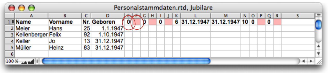
First, create a button that can be placed anywhere. In the button, the Formula F-3.9 is entered – as a formula and not as a command! This makes the button the trigger for the formula in the cell «Anniversaries!F1» (see Fig. F-3.5).
First, create a button that can be placed anywhere. Enter the Formula F-3.9 in the button – as a formula, not as a command! This makes the button the trigger for the formula in cell «Anniversaries!F1» (see Fig. F-3.5).

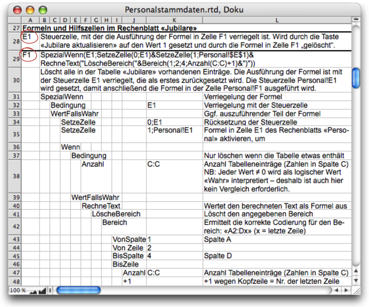
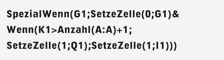
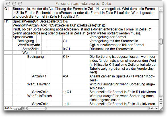
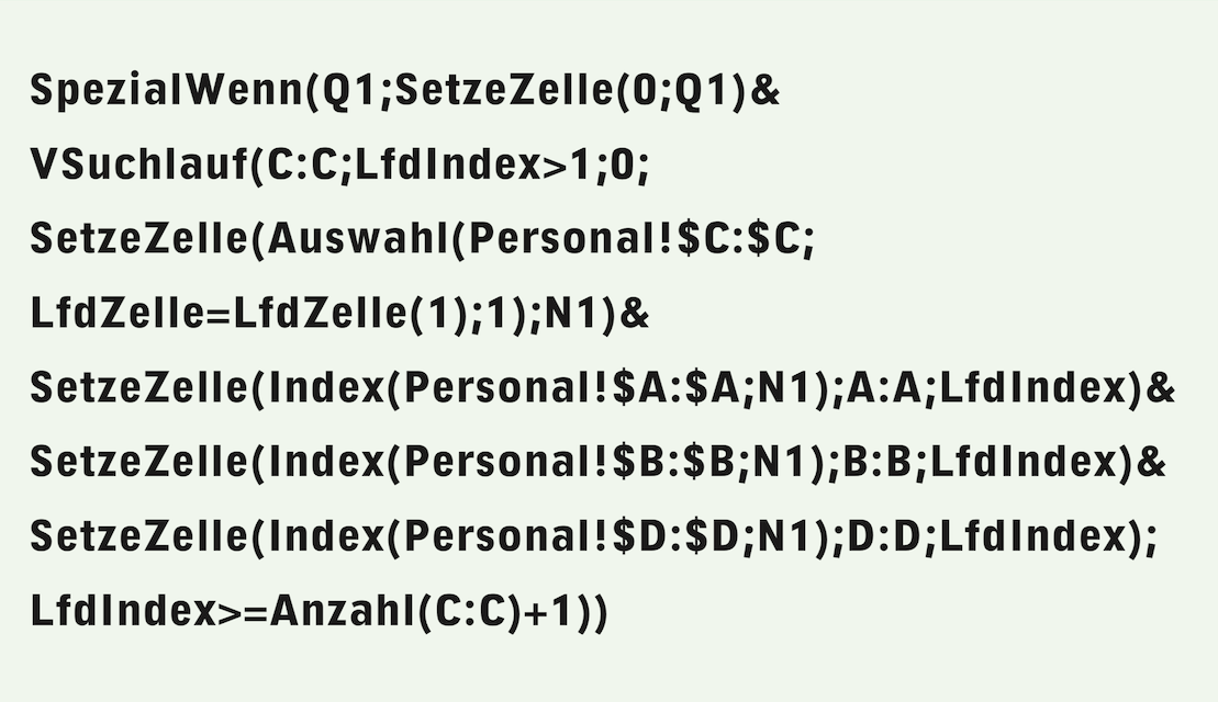
In cell «Anniversaries!F1», the «Search»/«SetCell» formula (see Formula F-3.10) begins with a preceding SpecialIf function. (NB: While reviewing this text, Jürgen Schell noted that in this case, «If» could also be used instead of «SpecialIf». But all the screenshots had already been taken.) This ensures that the remaining calculations are only performed if there is a 1 in cell E1. Let's take a closer look at Formula F-3.10. It is already made up of several sub-formulas, which are concatenated using the & operator. The documentation in Fig. F-3.6 helps us to understand it.
If the condition is met (a 1 in E1), the «SetCell» function immediately replaces this 1 with a 0. This ensures that the formula is only evaluated once! At the same time, however, the rest of the formula is also processed. The fact that the condition in the formula is not «E1=1» but only E1 is not a misprint. The value 1 also stands for the logical value «True» for the fulfillment of a condition and can therefore be queried directly with a reference to the cell without comparison. The subsequent «SetCell» command triggers a process in the «Personnel» spreadsheet, transferring the personnel data of the anniversary celebrants to the corresponding spreadsheet. But first, and this is the purpose of the rest of the formula, any old anniversary tables that may still exist must be deleted.
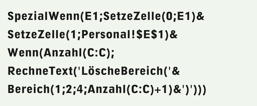
Of course, this is relatively easy to do with a delete range command. But how big is the range? The «Count(C:C)» function determines the number of existing table entries. If the table is already empty, this function returns the value 0 or «False», and the rest of the formula is not executed at all thanks to the If function. Note that no comparison is used for the condition here either. RagTime interprets not only the value 1 as logically «True», but all values except 0. Only thanks to the function «Range» (from the «Power Functions” extension) is it possible to calculate the range coordinates. Unfortunately, this function cannot be used nested within the «DeleteRange» function. This can only be achieved with a trick: this entire part of the formula must be compiled as text and then evaluated with the meta formula function «CalculateText». With four table entries, the calculated text results in the following formula, which becomes part of Formula F-3.10:

Now the anniversary table is ready to accept new entries. These must be searched for in the personnel table and transferred to the anniversary table. The corresponding formula is located in the «Personnel» spreadsheet, cell F1, and is locked with the control cell in E1, which was activated in Formula F-3.10.
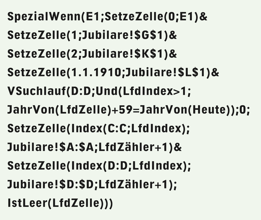
Here (Formula F-3.12) is the entire formula, which is documented in Fig. F-3.7. We used the function «VSearch» instead of «Search». The functions «Search» and «VSearch» or «HSearch» are interchangeable if only a single column/row is searched. Intuitively, we chose «VSearch» here because one column was to be searched.
We do not need to explain again the mechanism of resetting this activation and unlocking the next subformula by activating the cell «Anniversaries!G1». For the sake of completeness, here is the difference if the «If» function were used instead of «SpecialIf»: if the control cell blocks the execution of the formula, «SpecialIf» leaves the content of the cell with the formula unchanged, while it is deleted when «If» is used. The two «SetCell» commands of the “locking mechanism” are followed by two more, which enter initial values for a subsequent processing step in auxiliary cells of the anniversary table:

We will return to these when explaining the next step.
The search function is basically the same as in our example with the delivery note (Much more than just counting). However, in this case, the selection criterion is not simply a date in another column of the same row. In our case, the dates of birth in column D of the «Personnel» spreadsheet must be compared with today's date. The easiest way is to extract the year from the dates of birth and today's date using the «YearOf» function, as shown in this subformula:

Each match found is an anniversary celebrant whose personal data must be transferred to the anniversary table. This is the task of the last part of Formula F-3.12, i.e., «NextValue» and «AbortCondition» according to the syntax of the «VSearch» function. In contrast to other applications of the function, we are not interested in the «NextValue» as such. Rather, we are interested in the formula that is executed for the «NextValue». These are two «SetCell» commands.
For the time being, the personnel data does not have to be transferred in its entirety, as the anniversary celebrants still need to be sorted in ascending order of their birthdays. For this purpose, the personnel number as a unique identifier and the birthdays are sufficient. To prevent the values from interfering with the sorting process, we temporarily store the personnel numbers in column A of the anniversary table. The values are taken from the personnel list using the index function. The number of the row in which they must be inserted in the anniversary table is determined by the number of anniversaries already found. This is provided by the «CurrentCount» function, another function that can only be used within search runs.
The search is terminated when the first empty row in the personnel table is found. This means that one row too many is examined. To avoid this, we could use the «Index» function with «IsBlank(Index(D:D;CurrentIndex+1))» to look ahead one row. However, this does not offer any advantage in this case. In other cases, however, it may be important that no row too many is included in the search, especially if the «NextValue» is of interest.
With the specified Formula F-3.12, the value of the search function will be a value error because «YearOf(Empty cell)» does not return a valid value. With the alternative termination condition for the search, it would be a sequence of the values transferred with the «SetCell» commands at the last hit. Neither of these is of interest at this point.
To avoid confusion when displaying this function value, we select the «Nowhere» option for the «Spreadsheet Information ➝ Cell Contents ➝ Visibility» We do the same with all other “formula cells” in this example. However, it should be noted that the cells should be protected so that the completely invisible formulas are not accidentally deleted. In our example, we have also highlighted these cells in red for better identification in Fig. F-3.4 and Fig. F-3.5.
Can the effort we are going to put into solving this problem be justified at all? Of course, we could have transferred all personnel data to the anniversary table during the last search. A table created in this way can then be easily sorted by date of birth using the menu command. Transferring the data using the SetCell command has the advantage that there are no formulas in the table that could cause problems when sorting.
But here we want to assume that the document must also be usable for computer novices. So everything should run automatically, including sorting! The effort we have to put into creating the formulas is really only justifiable in exceptional cases. But here we are concerned with showing the way that must be sought in this case. That is why we want to make the effort.
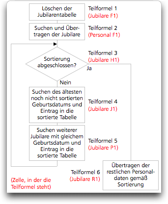
How does this sorting process work? Take a look at the flowchart (Fig. F-3.8), which shows the process schematically.
We have incorporated the formulas directly into the spreadsheets containing the data. Of course, they could also be placed in a separate spreadsheet. However, this would make them significantly longer and therefore more difficult to read due to the additional external spreadsheet references required. It is also convenient to be able to access formulas and values in the same window, especially when testing formulas. However, this approach is less practical for complex documents and tables.
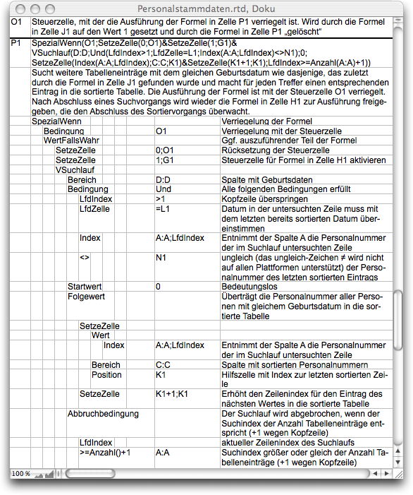
Now let's move on to Formula F-3.15 in cell «Anniversaries!H1», which is referred to as subformula 3 in Fig. F-3.8. The execution of the formula is locked in the usual way with the value of cell G1, which is activated by the second «SetCell» command in subformula 2 in the «Personnel» spreadsheet (Formula F-3.12). It is relatively easy to interpret. Nevertheless, for the sake of completeness, the documentation according to Fig. F-3.9 is also provided. In various steps of the process, values must be stored in auxiliary cells. In subformula 4, for example, the last birthday that has already been sorted and its position in the anniversary table must be known so that the next one can be searched for and entered in the correct place in the table.
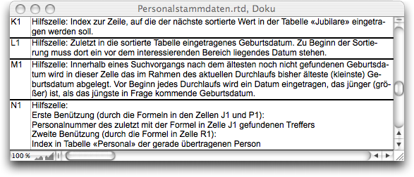
These values must be specified for subformula 4 in the first pass. This is the task of the two «SetCell» commands shown in Formula F-3.13. These are included as a subformula in Formula F-3.12. The purpose of these auxiliary cells (K1 and L1) can be found in the documentation in Fig. F-3.10.
The auxiliary cell K1 is also used in Formula F-3.15 to determine whether all items contained in the table (according to column A) have been sorted and the sorting process is thus complete. Depending on this, one of the subformulas 4 or 6 according to Fig. F-3.8 is activated.
We first follow the sequence of the sorting process, i.e., subformula 4 according to Fig. F-3.8 and documentation in Fig. F-3.11. Locking and triggering the next subformula are now self-evident. Before the search is started, the auxiliary cell M1 (see Fig. F-3.10) must be initialized to a date that is definitely after the earliest possible birthday – as a comparison value for the first birthday examined.
Three criteria must be met as «Conditions» for the search run: The row being processed must not be the header row of the table, the birthday being examined must be younger than the youngest one found so far (in auxiliary cell L1) and older than the oldest date found so far in this search run, which is contained in auxiliary cell M1.
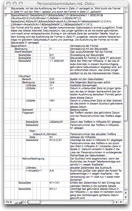
If the condition is met, the first of three «SetCell» commands replaces the date in auxiliary cell M1 with this date. The second command stores the personnel number of this hit in auxiliary cell N1 and also enters it in the anniversary table, column C, in the row where the next anniversary is to be entered, even though it is not yet certain that the person just found is the anniversary person. If an older, not yet sorted anniversary is found later in the search, this personnel number is overwritten again.
As a termination condition for the search, the number of personnel numbers in column A is checked to see whether all anniversaries have been processed. In this case, it is important that no extra rows are processed.
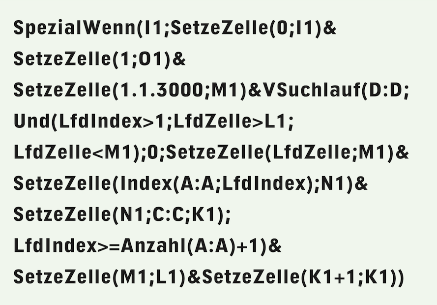
Did you notice that each time this formula is executed, only one anniversary employee, or rather their personnel number, is sorted? After the search is complete, two further «SetCell» commands are executed. The first increases the index to the anniversary table (auxiliary cell K1) by 1 so that the next time this subformula is executed, the personnel number of the anniversary employee found there is written to the next row. The second writes the date of birth found to auxiliary cell L1. It is indeed a complicated formula for sorting a single anniversary employee.
It's not just twins who have birthdays on the same day. This can also happen to employees of a company. And just because we have found one person with birthday X, we must not forget the others with the same birthday. This is the task of subformula 5 according to Fig. F-3.8 or Formula F-3.17. This, in turn, does not trigger the formula further to the right in cell R1, but rather subformula 3 again, by writing a 1 in cell G1. Formula F-3.17 is somewhat simpler than the previous one, but very similar in structure. See also its documentation in Fig. F-3.12.
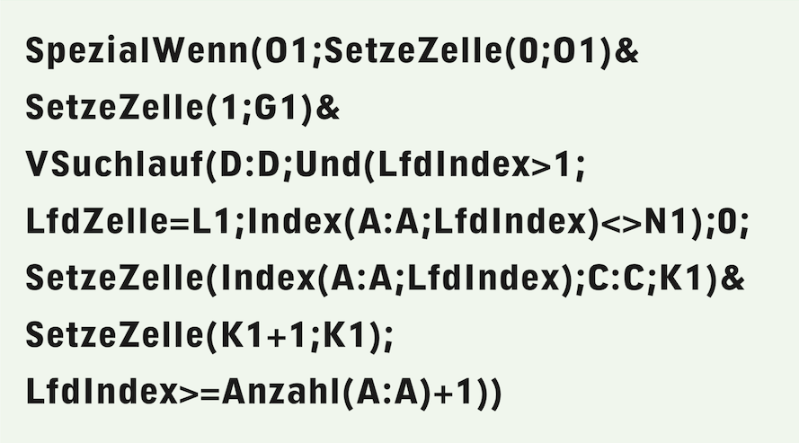
However, the condition is quite different. Of course, the header row must also be skipped here. The birthday of the row being examined must be the same as the one found in the last sorting step. And the personnel number must not be the one from this last entry, which is stored in auxiliary cell N1. We do not want to enter the same birthday boy or girl a second time.
The entry of the “twin anniversary” found is made in the same way as in Formula F-3.16: personnel number in column C, row according to index in auxiliary cell K1, which is then increased by 1. It is important, of course, that this formula finds not just one birthday boy with the same birthday, but as many as there are.
The termination condition for the search is the same as in the last subformula. After executing this step, the process returns to subformula 3, which checks whether the sorting process has been completed. Otherwise, the steps according to subformulas 4 and 5 are repeated until the sorting is complete.
If we now look at the result of the sorting, we see that so far we have only sorted the personnel numbers in column C of the anniversary table in the correct order. We now need to add the remaining personnel data. This is the task of subformula 6, or Formula F-3.18, documented in Fig. F-3.13.
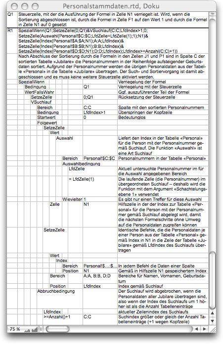
Since this is the last subformula of the sorting process, no further formula needs to be unlocked in this formula. As «Condition», the search only needs to consider the header row. This means that all other rows in the anniversary table are processed. For each row, the personnel data (last name, first name, and date of birth) must be retrieved from the personnel table according to the personnel number contained in column C. The same index is therefore required three times, which must be determined based on the personnel number. It makes sense to calculate this index only once and store it in an auxiliary cell – cell N1 is used. The calculation is performed using the «Select» search function, which has been available since the early days of RagTime. It returns the index of the row in the personnel table that contains the personnel number being searched for. The «Select» function is used within a search run. The «CurrentCell» function is used for both functions here. It must therefore be specified in the inner nested function that in one case it is the «CurrentCell» of the outer nesting level. The nesting index of the inner function is 0 and does not need to be specified, while that of the outer function is 1. Theoretically, even more nesting levels would be possible. However, we have not yet encountered a meaningful (and comprehensible) application of more than two levels.
Once the index of the personnel data to be transferred has been stored in auxiliary cell N1, three virtually identical «SetCell» commands follow, which transfer the data in columns A, B, and D from one table to the other. The termination condition is analogous to that in the previous formulas, except that it is now based on the number of personnel numbers in column C.
You probably worked up as much of a sweat following this sorting process as the authors did writing it. You may be wondering whether using the search function is really the best solution. We are convinced it is!
There are certainly other solutions for the task of creating the anniversary list. However, using «VSearch» – in another case it could also be «HSearch» or «Search» – has significant advantages, especially when compared to a solution based on formulas copied down in tables: the personnel list can be supplemented as desired without having to check any formulas, and the table can be copied, pasted elsewhere, and edited there, as no formulas are stored behind the values. Master the search function – it's worth it! Soon you'll be happily “building” searches yourself!
Let's not forget the simplest form of search: with two arguments, the range and the condition, searches – regardless of type – only count how often the condition is met in the range. The value of the function corresponds to this number at the end. The other two forms, with or without a termination condition, do not differ significantly. However, it is advisable to use a termination condition in case of doubt. It is easy to forget that the formula for the «NextValue» uses a function that produces an error with empty cells, for example. There have been several forum posts criticizing supposed search errors that were only due to missing or incorrect termination conditions.
It is important to make a distinction that is not apparent from the syntax: Is the search intended to determine a «NextValue», as in the example with the total of delivery note items delivered on the key date (Fig. F-3.1), or is it intended to execute processing steps – usually using «SetCell» – in which the «NextValue» as such, and thus the value of the function after its execution, plays no role at all. In the latter case, it is important to note – a problem we have not encountered here – that the formula for the «NextValue» can be processed in such a way that no errors occur.
Type conflicts in the processed data are most likely to lead to such errors. If an error is detected during a search step, the search is aborted. Such errors are not easy to track down!
After studying the example with the sorting process, you will surely agree with us: search runs enable script-like constructions that further enhance the already high performance of RagTime. Take advantage of this!
The mail merge function is actually also a search function! This is often overlooked. The function «CurrentCell» can therefore also be used in arguments. If we want to send an invitation to the anniversary outing only to all anniversaries who turn 60 this year, and are not interested in a separate, sorted table at all, then for personnel master data arranged according to Fig. F-3.4, we could also work with «MailMerge». It is important to realize that if several mail merge functions occur in the same document, all «SelectionConditions» must always be met for the relevant “data record” to be printed. This allows us to split the formulas. So if in your letter with the formula
The mail merge function is actually also a search function! This is often overlooked. The «CurrentCell» function can therefore also be used in arguments. If we only want to send an invitation to the anniversary outing to all those celebrating their 60th birthday this year and are not interested in a separate, sorted table, we could also use «MailMerge» for personnel master data arranged according to Fig. F-3.4. It is important to realize that if there are several mail merge functions in the same document, all «SelectionConditions» must always be met in order for the relevant “data record” to be printed. This allows us to split the formulas. So if you use the formula

in your letter to retrieve the name from the personnel master data and use another column reference for the other elements, you can use the following formula
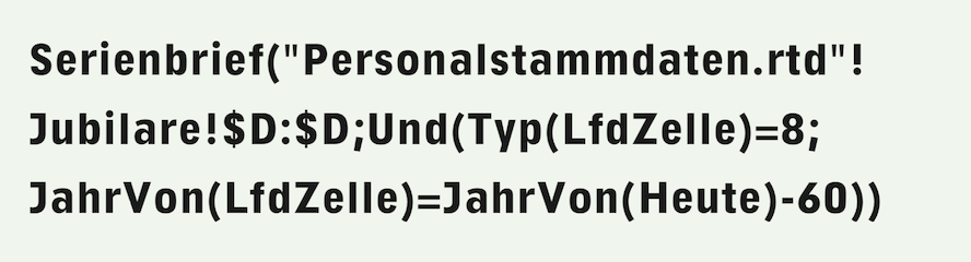
to specify the selection criteria for the people who are to receive the letter. The first of the conditions linked with «And» in Formula F-3.20 excludes all rows that do not contain a date in column D, i.e., the header row and the empty rows. The second condition selects all persons who will turn 60 this year.
The formula can be placed anywhere in the text, with graphic text on the page, or in a spreadsheet that does not appear in the layout at all. If the formula is placed in the text or on the layout page, you should assign the resulting text to “non-printing fill” – otherwise, the date of birth will suddenly appear somewhere on every letter!
The function «CurrentCell» is used in the above Formula F-3.20. ‘Spaltenwert’ would also be permissible, but not the other special functions that can only be used within search runs. For more information on form letters, see section 2.5.6 “Mail merge with selection”.
The «Select» function was already available in RagTime 3, where it served as a “search run”. But it is actually also a search run function! The same special functions are permitted in its arguments as in the mail merge function. Unlike search runs, «Select» can be used to find the nth hit very directly (in this example, the nth row containing the value 1 in column A is searched for):

The syntax is simpler than for the equivalent search:

As long as there is an nth hit, both formulas deliver the same result, namely the index of the row with the nth hit. A subtle difference arises when there are fewer than n hits in the searched table.
Formula F-3.21 with the selection function then correctly returns the error value “NV!” (= Not available), while Formula F-3.22 with the search run function returns the index of the last match found. This can lead to errors that are difficult to locate. Therefore, always use the «Select» function when searching for the nth occurrence of a value in a table and check for errors!
● Break down complex processes into subformulas that are locked with control cells and «SpecialIf» or «If». ● Do not place formulas and auxiliary cells on rows with table values, but in the header of your table – or in another spreadsheet. ● Avoid using the «ColumnValue» (or «RowValue») functions with «n» as an absolute number, thereby avoiding errors when inserting columns and rows – use «Index» instead, even if this is a little more time-consuming. ● If you still use the «ColumnValue» function, note that the referenced column must be within the search range specified in the search function! ● Note the order of the conditions in searches! For example, if you search a column for a date and use a date function in the condition, an error will occur in the header if there is text there. The exclusion of the header with the condition «CurrentIndex>1» must therefore precede the condition with the date function so that it is not applied to the header at all. ● Complex sequence value calculations must not contain any type incompatibilities. ● Document your formulas. You do not have to use the documentation method shown here. However, your documentation should enable you to easily understand and comprehend your formula even after a long period of time, and you should adapt the documentation when changes are made!