2 RagTime at school

RagTime has been popular in schools from the very beginning. Here, with RagTime 7, we look at examples from a private school. What can be learned there is mainly how to organize the administration well. In addition to letters, mail merges, address lists, and scheduling, we also deal with handling buttons. It remains to be hoped that everything is prepared clearly enough so that you don't have to stay after school.

Our example with the school

The private language school “YesNon” is a franchise company with currently five schools: In London, Malta, Montpellier, Munich, and Zurich. All these schools participate in the success and are supported by the headquarters in Frankfurt in every respect. From here, marketing, quality control, and billing are also managed.

The school is aimed at young people between the ages of 16 and 26. A language stay lasts at least 6 months. During this time, you will study half the day and work half the day in companies or non-profit organizations. The qualification of an attended course is not limited to school language successes, but also includes social skills gained through practical work.

2.1 Letterhead or RagTime 7?

That is not an absurd question. Documents and writings are increasingly sent electronically. And ever better PostScript printers can produce appealing high-resolution print quality. Thus, the question of which papers actually need to be ordered from a printing shop is justified. A single sheet of multicolored paper may suffice, and everything else can be handled individually with self-designed forms. Because small and medium-sized businesses, as well as self-employed individuals, can quickly and efficiently create their own RagTime stationery pads (with the suffix .rtt), we will first discuss the letter form. In the example of the language school, there are six different locations (e.g., Fig. 2.1 in Munich), which require well-prepared organization. An ordinary letter form will hardly suffice. Therefore, let's build a more sophisticated form step by step.

Fig. 2.1:

A letter form that “thinks along”

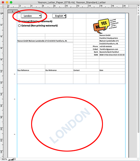
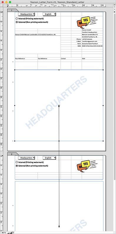
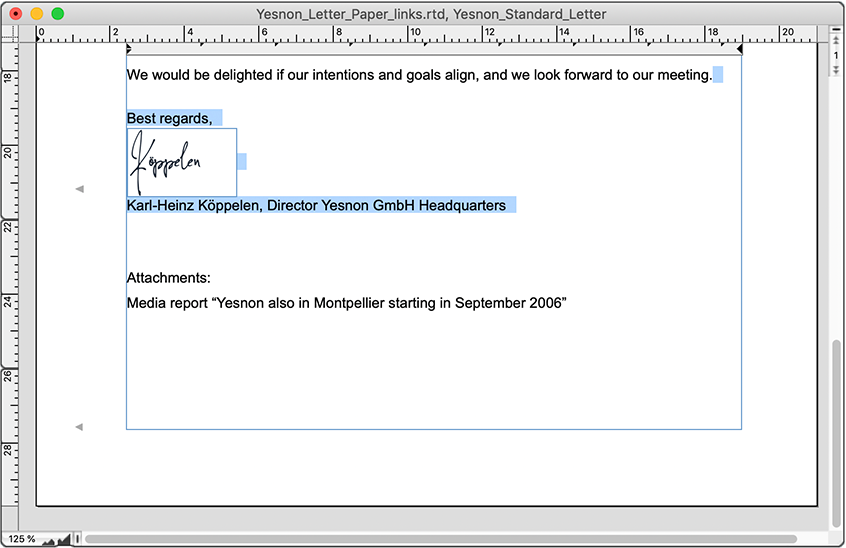
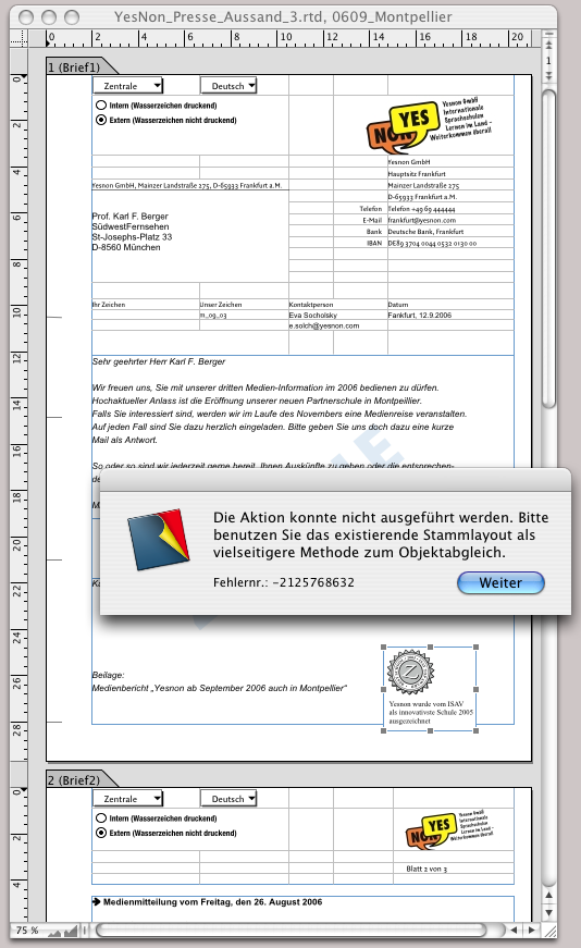
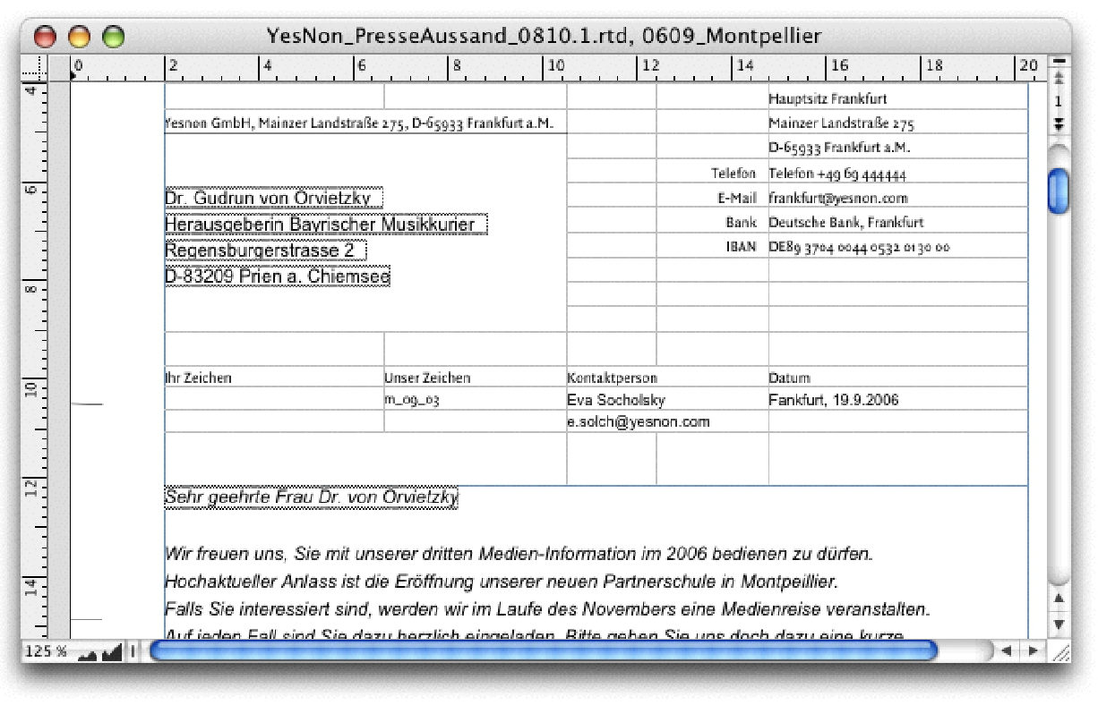
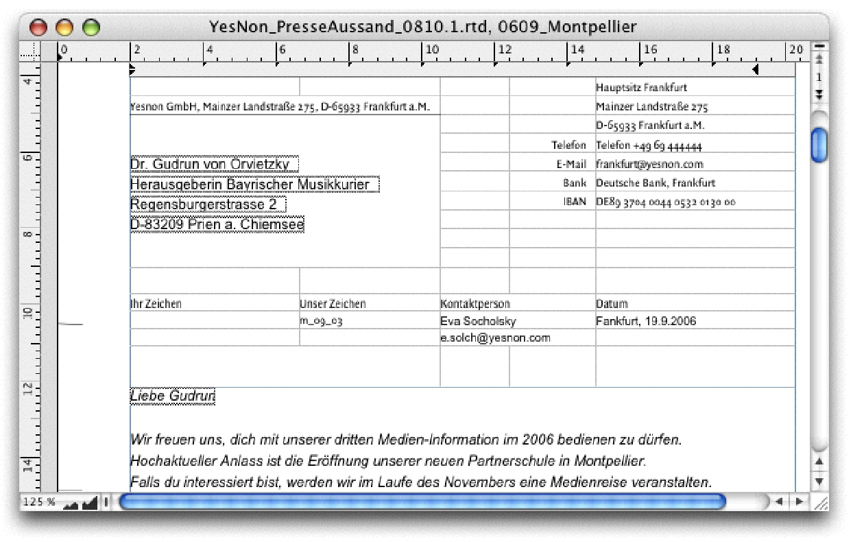
At YesNon GmbH, things are multilingual. All schools work with the same RagTime documents. It should be possible to decide individually at each workstation which language the letter or notice should have. For us, it is interesting to discover the possibilities that forms offer when they are built with spreadsheets (see Fig. 2.2). On the left, the document as it looks in daily use, on the right, the document with all non-printing elements retrieved from a stationery pad.

Fig. 2.2:

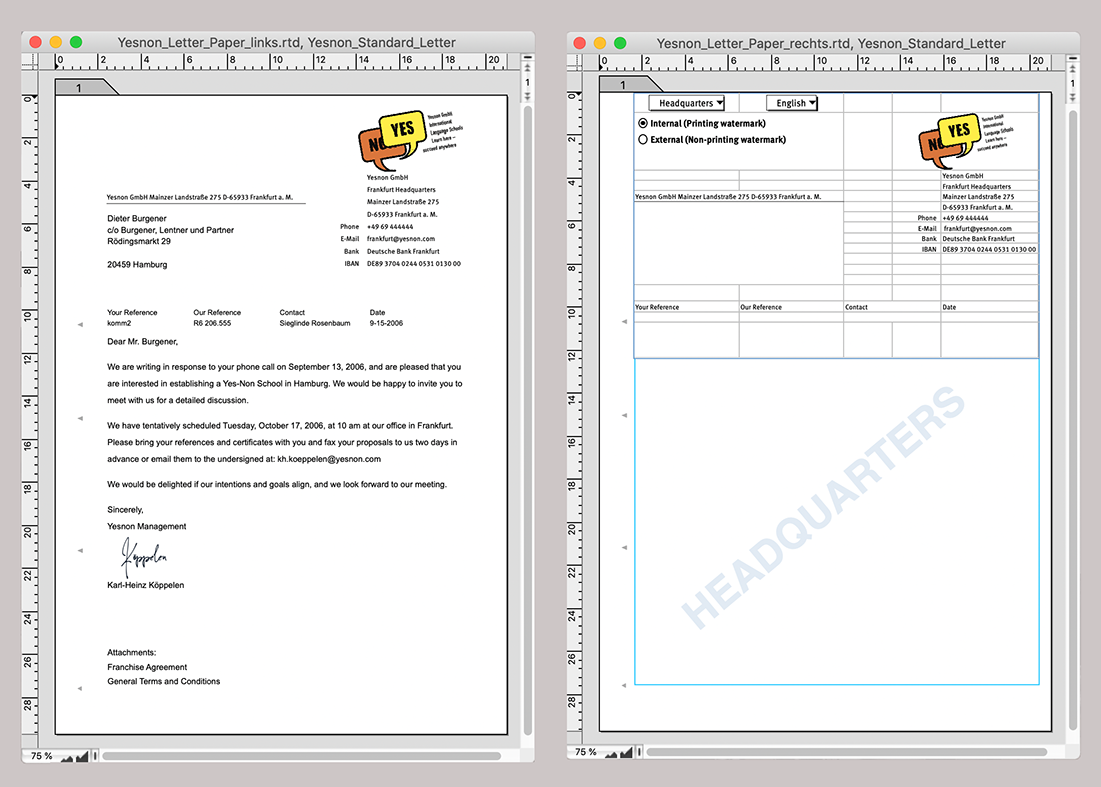
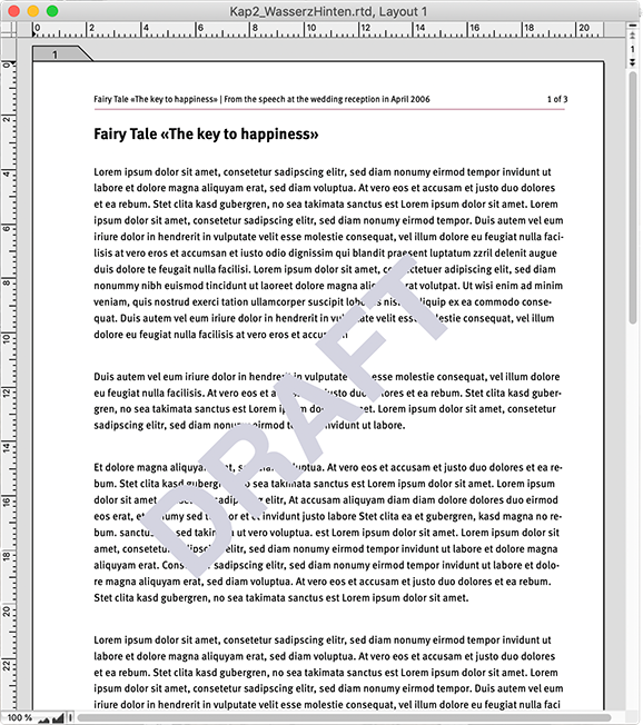
In this document, three things are particularly noticeable: First, the upper third is a spreadsheet (except for the fold marks), second, buttons are built in, and third, behind the text frame intended for the letter text, a watermark with the location designation «Head Offices» is visible. This watermark is linked to the first selection button and the radio buttons below it. This allows the user to specify at which location the document was created. Since such watermarks can be a great help in a wide variety of documents, we first turn to this function.

2.2 Watermarks as aids

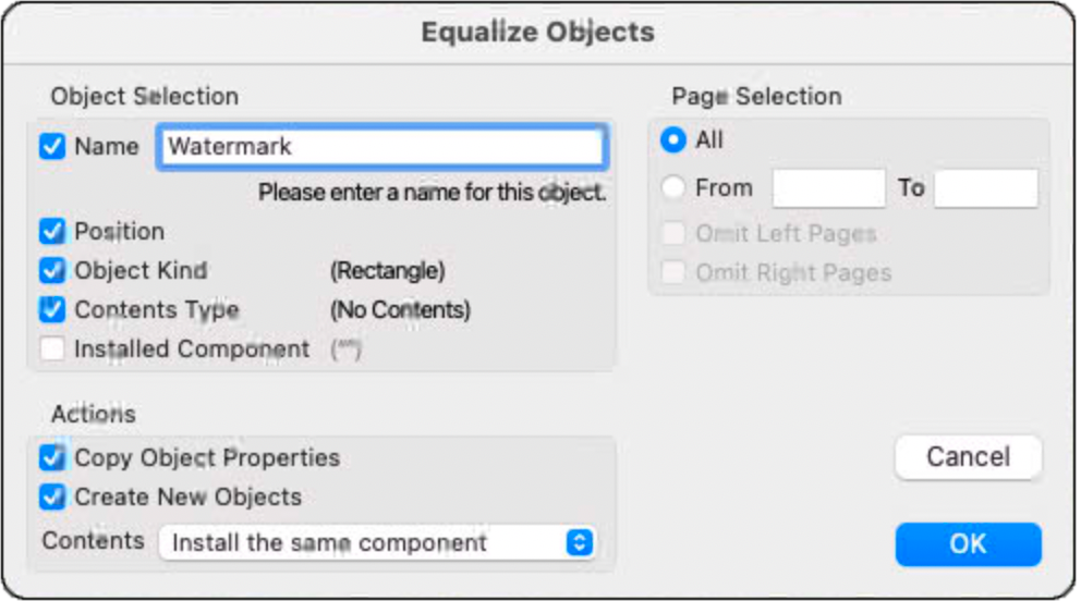
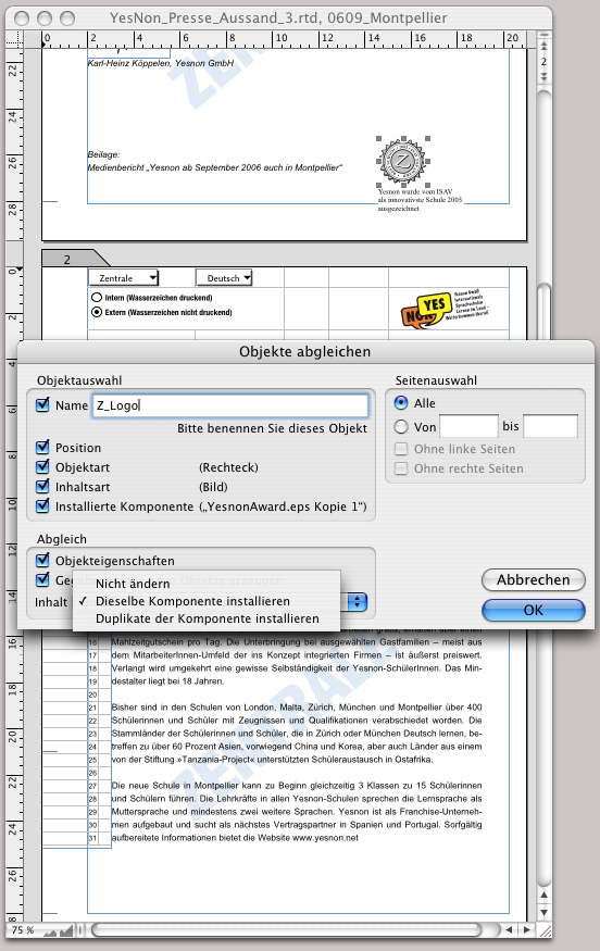
In long-term projects, there are often a lot of documents, and in several versions. Watermarks, possibly with dates, facilitate the overview. A simple watermark is built quite quickly: With the graphic text tool, write the desired text – in large font size and with light color or black and a tint of about 10%. Rotate the text line so that it runs diagonally across the page and then move the text element to the back («Drawing ➝ Stacking Order ➝ Send to the Back»). Draw a container over it, which is now on the front layer – and is usually defined as a text component in the layout. It must have a transparent fill style sheet. If it is a spreadsheet container, care must be taken that not only the container itself, but also the filling of the cells is set to «Transparent». With «Equalize Objects» (see Fig. 2.3), the element can be copied to all or the desired pages in one operation.

Fig. 2.3:

Fig. 2.4:

Fig. 2.5:

Not really a good solution

Sometimes the first solution is not really the best solution. As an exception, we have presented a very “spontaneous solution” to illustrate the system but it is not ideal in this case. The purpose of the «Equalize Objects» function is to either place individual components on several defined pages or to change them simultaneously. This is not suitable for variable texts, such as our watermark. We assume that the text of the watermark should change when a new version of the document content is created.

Watermarks on master layouts

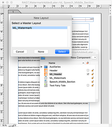
Master layouts have the advantage that elements inserted there – in our case graphic text – immediately appear on all pages of the layout that depend on this master layout. But what to do if the document has no master layout yet? Then simply create the master layout afterwards. It is best to open the Inventory of the document to better overview the processes. There, select under «New Component ➝ Master Layout» and give the new master layout a name right away, for example «Watermark». One page of the master layout is sufficient: there you can create the watermark with graphic text in a large, bold font. Create a fill style sheet with a transparent color «Windows ➝ Auxiliaries ➝ Fill Style Sheet Editor ➝ Opacity». An opacity of 10 to 15% should be sufficient. After that, only the existing layout needs to be linked to the new master layout. If the font now flows around the watermark text in the layout, select the graphic text element on the master layout and turn it off under «Information ➝ Objects ➝ Text Flows Around» (remove checkmark). Thanks to the transparent font, the text in the layout now appears to run over the watermark. In reality, the graphic text is on the frontmost plane on all pages and cannot simply be moved to a rear plane. Therefore, as a learning effect: A master layout can indeed be created afterwards, but it should also contain the essential elements for the layout to be able to correctly select the planes – for our watermark. Basically, the next section applies to all subsequently created master layouts.

Fig. 2.6:

Fig. 2.7:

2.3 Subsequent master layouts

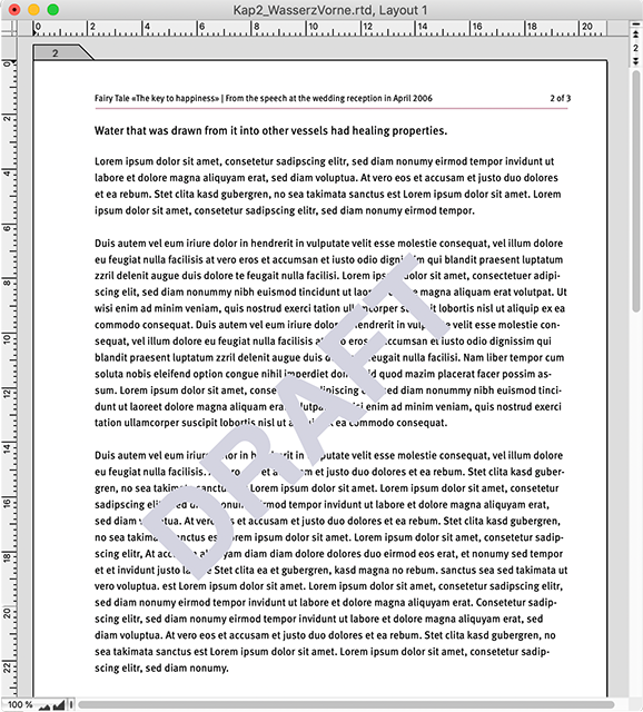
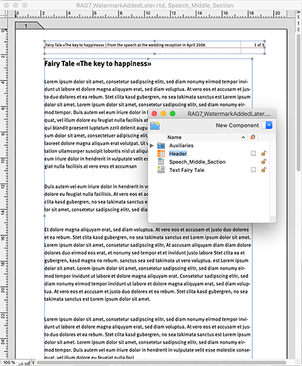
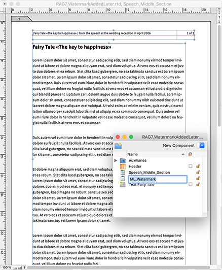
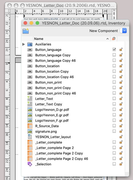
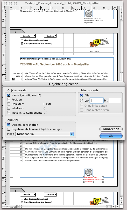
Fig. 2.6 shows the Inventory of the document, with the layout page in the background. The header as a spreadsheet, then the text component. In Fig. 2.7, it is visible that a new master layout has been created with the name «ML_Watermark». Select all components of the first layout page, e.g., with AA/6A, copy them and paste them into the master layout. The corresponding symbols and names of all copied components now appear in the Inventory. That shouldn't bother you: What is too much at the end can simply be deleted. Convert the text container on the master layout page: «Drawing ➝ Contents Type ➝ No Contents». This automatically deletes the copied text of this container. The empty frame still gets a pipeline for automatic page addition. Now enter the watermark text using the graphic text tool, rotate as desired, and set it to the rearmost plane (see Fig. 2.8). But attention: In the spreadsheet frame of the original layout, in cell B1 of the header, a formula for page numbering was entered. This no longer works with a master layout.

Fig. 2.8:

Fig. 2.9:

Fig. 2.10:

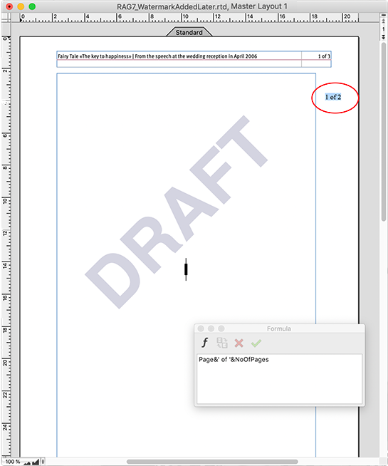
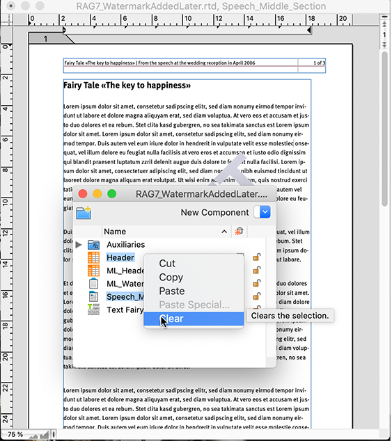
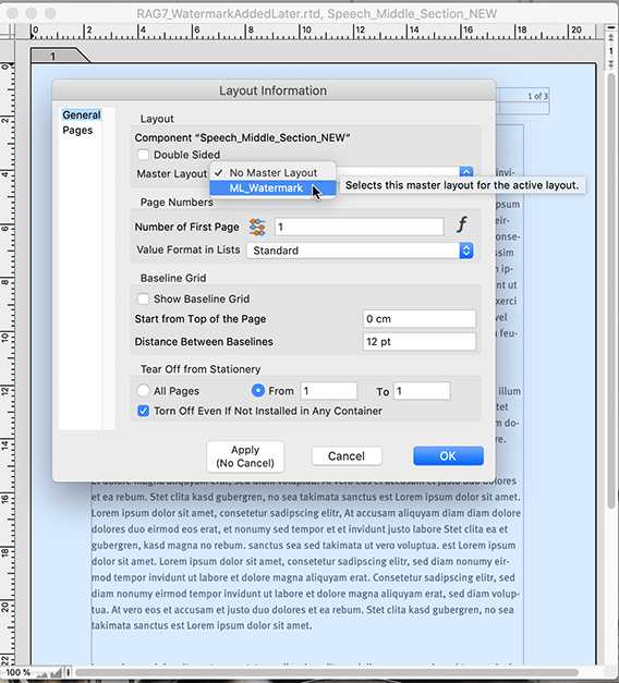
There the same formula must be inserted as graphic text. In the illustration, this text is circled in red. Drag the graphic text with the formula to the right place and delete the formula at this place in the spreadsheet: The master layout is finished. Now create a new layout from the Inventory. A question will pop up asking if it should refer to the master layout «ML_Watermark». That's exactly what we want – and thus a new layout dependent on the master layout is created (see Fig. 2.9). After that, there is nothing more to do than to drag the text «Fairy Tale Text» from the Inventory into the newly created layout. There now exists a completely new layout that looks just like the original layout, but is additionally linked to a master layout that has a replaceable watermark. All unnecessary components – the old layout and the old header – can now be deleted in the Inventory. Make sure that no checkmark is set for the text component, otherwise the whole fairy tale might be deleted. In this case, without triggering another action beforehand, choose the undo command – and away with the checkmark!

2.3.1 Detaching master layouts

In the page tab of your layout, you can double-click to open the layout information and detach the links from the master layout for the entire document or for individual pages. After that, all components can be moved freely in the layout again but the connection is gone and with it the possibility to make general commands or changes via the master layout.

Tip:: Watermarks can be useful in a wide variety of applications. Most often probably when it should be immediately recognizable in the document or on each printed sheet whether it is a draft, a “ready for printing” etc.

Upon re-linking with the master layout, the following happens: All components of the master layout are inserted into the layout again, on the frontmost plane. The existing components are overlayed which can lead to a frantic search for seemingly lost text. All components are now double-stacked, and since the command cannot be undone, this would result in time-consuming deletion of superfluous components. Generally, we recommend that whenever you want to “try out” something with master layouts, create a copy of your starting document beforehand.

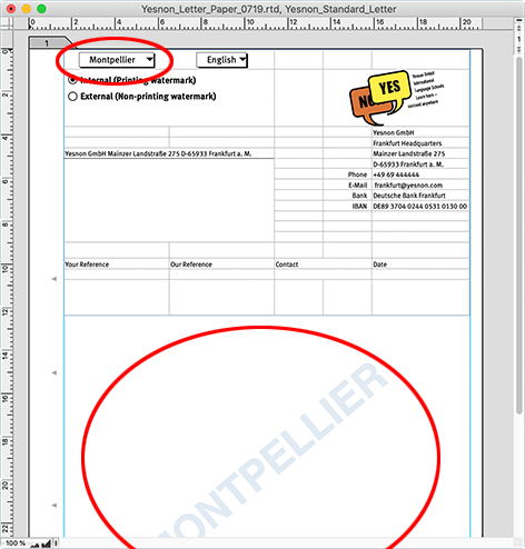
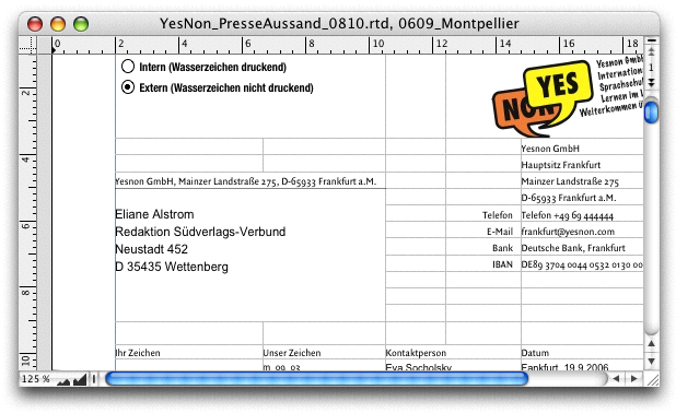
Intelligent watermarks with buttons

Let's go back to our document of the YesNon language schools. The watermark in the letter form changes depending on which school acts as the sender. At the same time, however, there are two watermarks: One that appears only in the document – as an internal identification mark when exchanging RagTime documents – and a second watermark that should also appear in the print and in the exchange of PDF documents (see Fig. 2.12/Fig. 2.13).

Fig. 2.11:

Fig. 2.12:

Fig. 2.13:

Fig. 2.14:

Fig. 2.15:

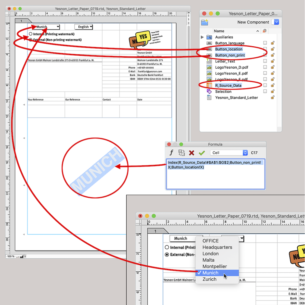
Although we go into more detail on the functions and creation of buttons in chapter “Formulas Part 2: Variety of buttons”, we want to delve a bit deeper here into the changing watermark and the buttons associated with it. In Fig. 2.14 and Fig. 2.15, the relationships between the buttons and the watermark are made visible. But this also requires a detailed explanation:

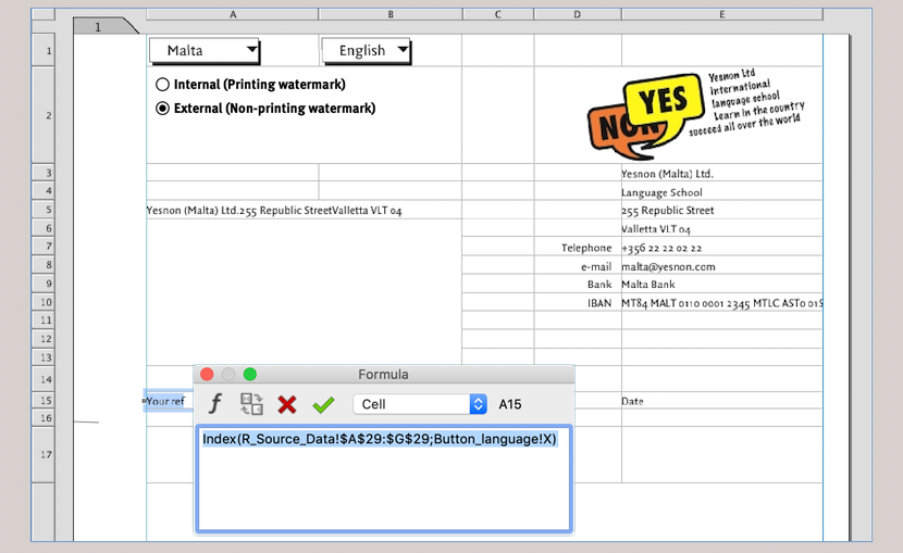
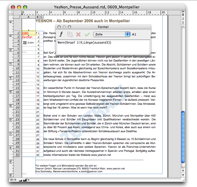
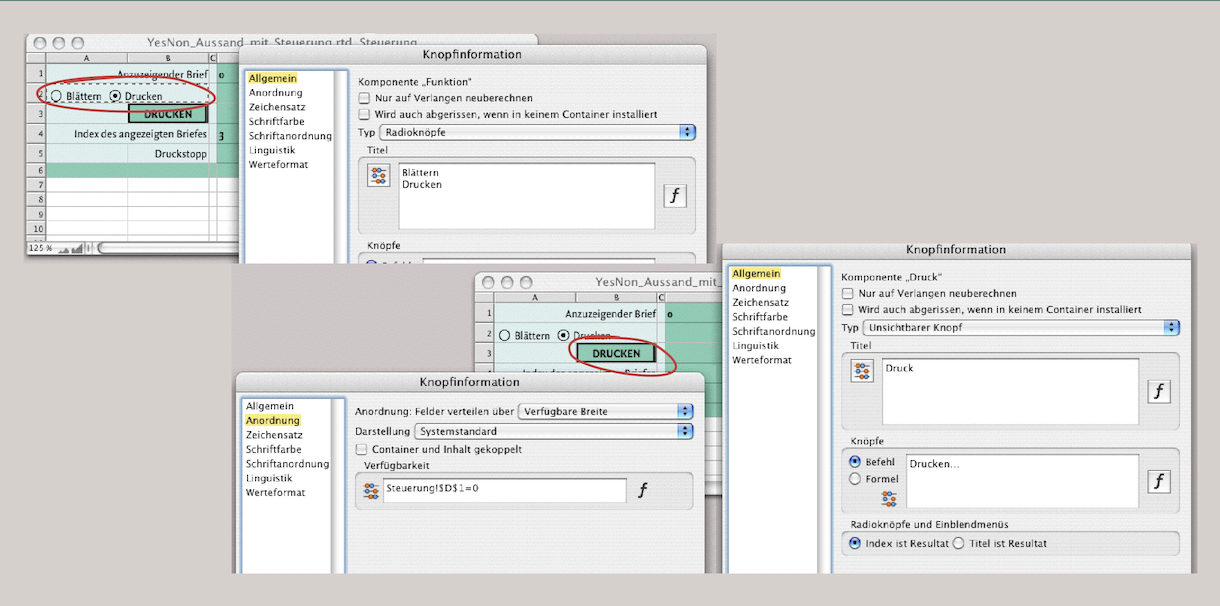
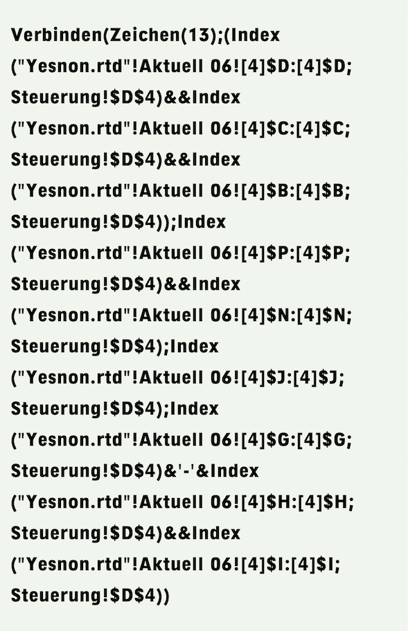
The button «Button_Location» controls the location designations in the watermark. To do this, it retrieves the corresponding terms in the already correctly formatted font from the spreadsheet «S_Source Data». The component that reproduces the watermark in the letterhead is a graphic text that merely contains a reference as a formula. The component was pulled large enough to be able to reproduce even the longest location name «MONTPELLIER» on one line. Rotating the component by -38° can also be done later. The formula to be entered is:

Formula 2.1:

The formula refers to the pop-up menu button «Button_Location» and to the radio button «Button_Nonprinting».

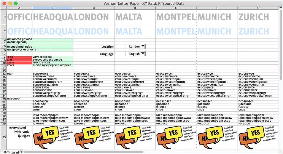
«Index» is the function that delivers the value of a spreadsheet cell from a specific range. The range A1:G2 includes the location names for the watermark in the spreadsheet «S_Source Data». The opened spreadsheet «S_Source Data» is displayed in Fig. 2.17. Row 1, from cell A1 to G1, contains the location designations formatted as printing, row 2, from cell A2 to G2, contains the location designations formatted as non-printing. The remaining contents of this spreadsheet serve another purpose in connection with the letter forms. We will come to that in the next section.

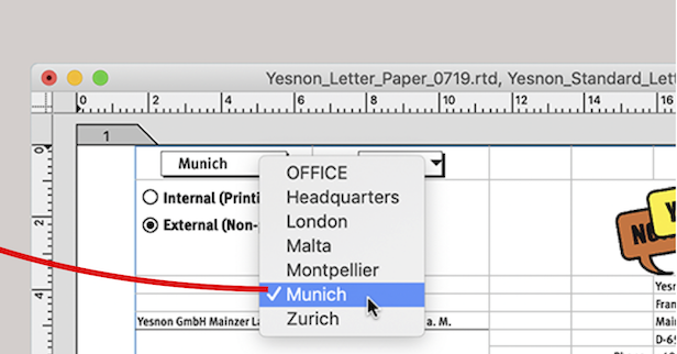
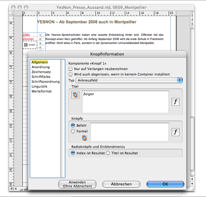
The second specification in the formula after the semicolon defines the line in this range. And this specification is provided by the button «Button_Nonprinting» (either row 1 or row 2). The third specification of the formula concerns the column in the range, provided by the button «Button_Location» (column 1 to 7, depending on the selection in the button. Compare Fig. 2.15, «Munich» corresponds to column 6). For the button «Button_Location», the following formula must be entered on the panel «Button Information ➝ General ➝ Title» (the button information is easiest to open with the pressed “/6 key and a double-click):

Formula 2.2:

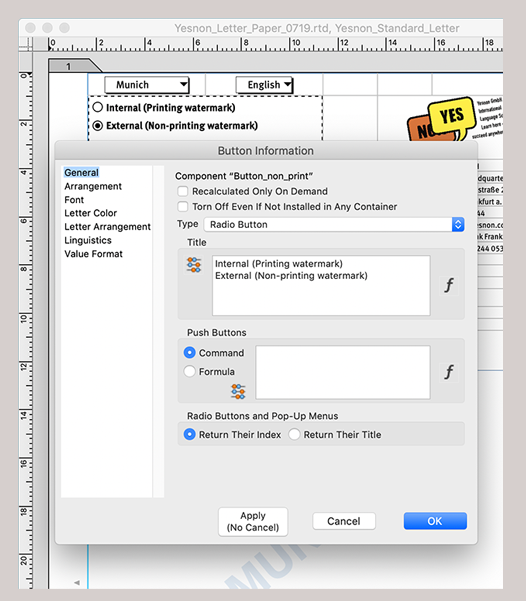
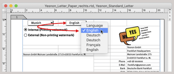
For the radio button «Button_Nonprinting» you only need the designations that should be selected for operation: «Internal (Watermark printing)» and «External (Watermark non-printing)» as evident in Fig. 2.16. With that, the watermark exercise is already finished.

Fig. 2.16:

Fig. 2.17:

If you want to use the components created in this way for other purposes (e.g., to mark manuscript versions), you only need to change the terms in the first two lines of the spreadsheet «S_Source Data». Starting from our YesNon letterhead, we have placed the two buttons just described in cells A1 and A2 of the spreadsheet «_Total Letter». You can of course name your corresponding spreadsheet differently, e.g., «Watermark».

The whole thing again in the master layout

Your watermark combination now consists of a spreadsheet, in it a pop-up menu button with the terms for the watermark and a radio button with the selection whether printing or non-printing. In addition, you have a graphic text with the reference to the actual watermark and a spreadsheet with the source data that already contains the terms correctly formatted. If you now place the graphic text on a master layout page and also the spreadsheet with the buttons (as a non-printing object), then you always have the right watermark on every layout dependent on this master layout and can change it from any page with the help of the buttons (otherwise, elements dependent on the master layout can only be changed in it itself. The change then affects all pages of your layout.

Fig. 2.18:

2.4 Multilingual letterhead

Let's return to our YesNon letterhead with the third button, the pop-up menu for language selection (Fig. 2.18). With it – together with «Button_Location» – the addresses, the reference notes, and the sender identification in the letter window should be exchanged. The same letter form is thus usable for all locations of the language school. This increases flexibility, as every user has all letter forms of the YesNon language school available at any time and can send letters on behalf of another school. The area of application of the solution shown here can be transferred, e.g., by switching a single form as letter, delivery note, invoice, reminder, etc. via pop-up menu. The principle remains the same.

Fig. 2.19:

Fig. 2.20:

Fig. 2.21:

Fig. 2.22:

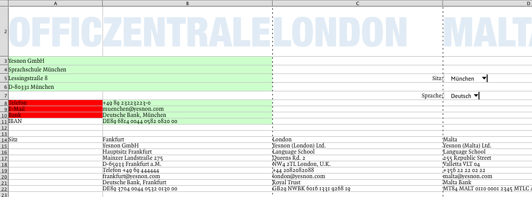
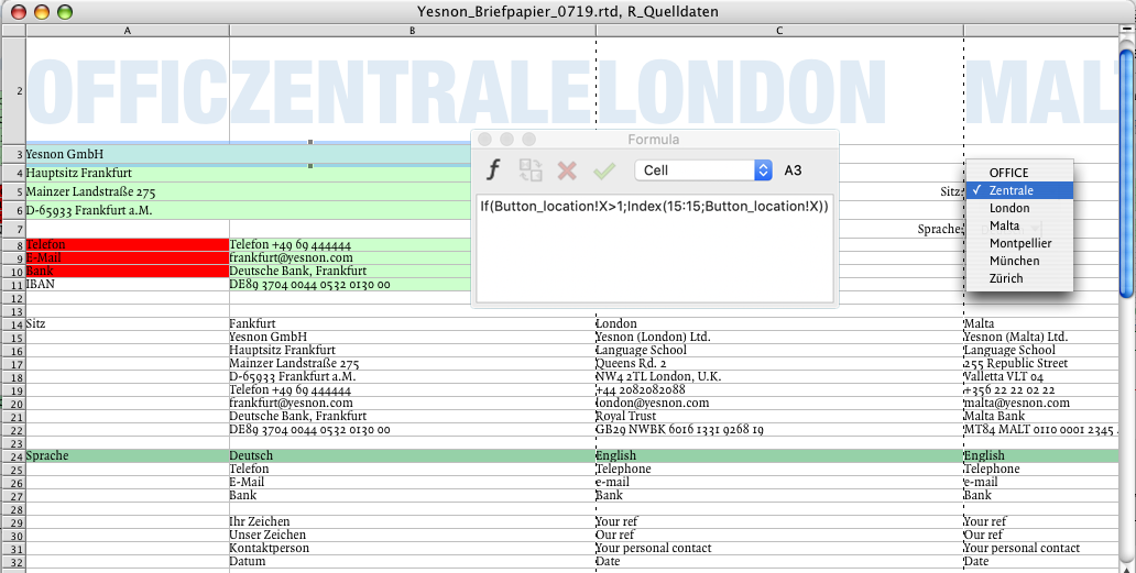
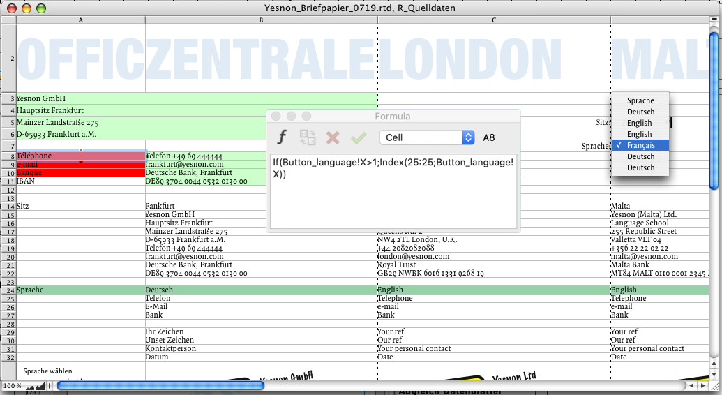
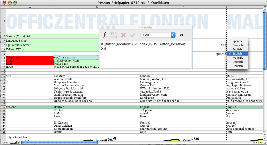
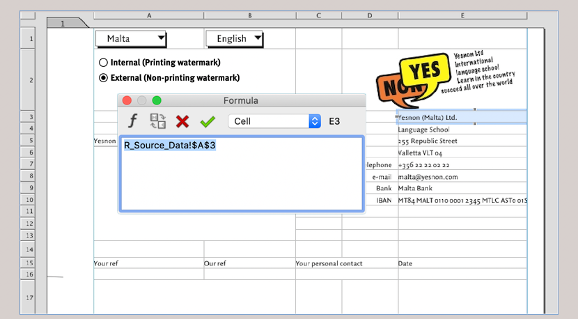
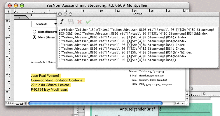
In Fig. 2.19, the spreadsheet «S_Source Data» is enlarged in a section. All cells underlined in red or green contain a formula. In addition, the discussed buttons are inserted here again to be able to check the correctness of the functions directly in the spreadsheet. In cells A3 to A6, the correct address is assembled from the six different company branches; this in relation to «Button_Location». The formula in cell A3 is therefore copied down to A6. So if one of the locations is selected with the «Button_Location» (Index > 1), then in cell A3 the correct company name is fetched from row 15, in cell A4 the correct sub-designation from row 16, in cell A5 the correct street from row 17, and in cell A6 the correct place from row 18. According to the same logic, cells A8 to A10 are about the correct language and cells B8 to B11 about the respective phone numbers, email addresses, bank details, etc. Needless to say, these color-marked cells are then referenced accordingly in the spreadsheet «_Total Letter». In Fig. 2.23 to Fig. 2.26, these references are made clear. The formula shown in cell E3 applies with the corresponding reference to all parts of the letterhead.

Fig. 2.23:

Fig. 2.24:

Fig. 2.25:

Fig. 2.26:

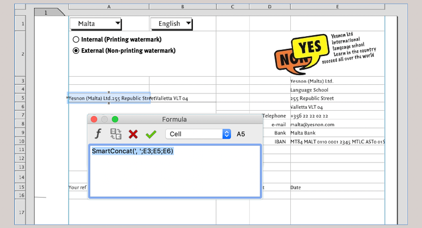
With the function «SmartConcat» the sender identification for the address window references the addresses. This allows several cell contents to be connected to a text that is strung together by certain recurring characters. In our case, that is a comma and a space (Fig. 2.24).

The signature characters and the logo, which differs in each language, in Fig. 2.25 and Fig. 2.26 refer back to the «R_Source data» spreadsheet with an index function and the pop-up menu button «Button_Language». Thus, a comfortable and user-friendly letter form has been created, which can be supplemented with a following page and saved as a RagTime stationery pad (with the ending «.rtt»). Let's stay with the topic of master layout in the next section – and with the difference to the form, which can also depend on a master layout.

Fig. 2.27:

Fig. 2.28:

Form or master layout?

Those who are not very familiar with RagTime often have trouble deciding for one or the other solution. Therefore, here are a few thoughts on advantages and disadvantages: In a form with a ring pipeline, pages are automatically added when the text overflows on a page. The objects on the individual pages are independent of each other. This can be an advantage or disadvantage. If the same object – e.g. a logo – appears on all pages, then in the form, each logo is a new copy. That can really inflate the Inventory (see Fig. 2.29). In addition, in a form without master layout, all pages that become superfluous due to text shortenings must be deleted by hand again. Otherwise, the form is sufficient for simpler, less extensive layouts.

Fig. 2.29:

Fig. 2.30:

However, form and master layout do not exclude each other – if a form is based on a master layout, all advantages are combined! In the form with master layout, not only are pages automatically added when text lengths change, but unnecessary pages are also automatically deleted. In addition, the components that depend on the master layout are the same on all layout pages (thus not as copies). Thus, you can also make changes on all pages simultaneously via the master layout. However, if you want to change individual components on a page in the layout (be it in arrangement or size, etc.), these pages must be detached from the master layout. But with specially adapted master pages, almost every wish for different page design can be realized. More about that in chapter 3 “Ready for print by notes”.

Preparing a media mailing

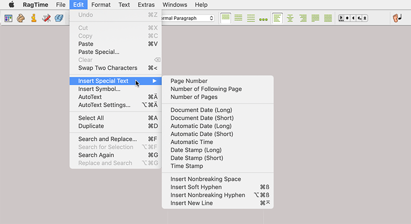
From the YesNon headquarters in Frankfurt, a mailing to selected German-language media is planned: A press text and a personal cover letter, of course based on our letter form. In the context of this task, we can address some special features in advance that RagTime offers in connection with text creation and text corrections. Under «Edit ➝ Insert Special Text» there are a whole series of special texts that can be inserted at any point in text components (or texts in other component types) (Fig. 2.30).

Insert special text

Only the date and time special texts require explanation. With «Date Stamp», the date is inserted as fixed text, with «Automatic Date» as a date updated with each document use, and with «Document Date» as the date of document creation, or of the tear-off from the stationery pad. The time special texts are to be interpreted analogously. The document date can, if e.g., a letter is only sent the following day, be changed in «Extras ➝ Document Settings… ➝ Document», but remains, apart from this change possibility, fixed in the document.

The insertion of a special text is simple: The special text is inserted where the insertion mark is flashing. Behind all special texts is a formula – so it is calculated text. If you select «Windows ➝ Show ➝ Formula Borders in Text», all these texts are framed with a fine dotted line. Of course, a special text can be deleted again or moved to another text position, but within the special text, for example in an automatic date, nothing can be corrected or changed. In any case, you can subsequently assign a different value format to a date special text – except for the date stamp, which stands as text in the formula.

Insert symbol

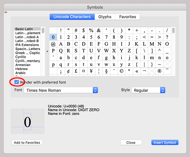
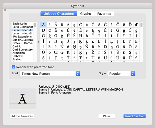
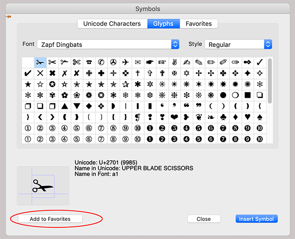
«Edit ➝ Insert Symbol» opens a window that makes all fonts and characters available on your computer usable. Under «Unicode Characters» (see Fig. 2.31), you can scroll left or right to find the desired character ranges. This way, foreign language characters and symbols can also be found and inserted. The panel «Glyphs» (Fig. 2.33) is not quite aptly named. The term «Glyphs» denotes variants of types in typography, mainly in ornamental and script fonts. Here, «Glyphs» is an generic term for all special characters.

What makes «Insert Symbol» so interesting are two points: First, all characters can be inserted directly matching your currently selected font formatting. For this, the checkmark must be set (see red circle). Second, you can add all characters with «Add to Favorites» to the «Favorites» panel, where you can assign them a keyboard shortcut, thus a kind of «Alias» (Fig. 2.33, Fig. 2.34, Fig. 2.35).

Fig. 2.31:

Fig. 2.32:

Fig. 2.33:

Fig. 2.34:

Fig. 2.35:

Fig. 2.36:

Fig. 2.37:

Fig. 2.38:

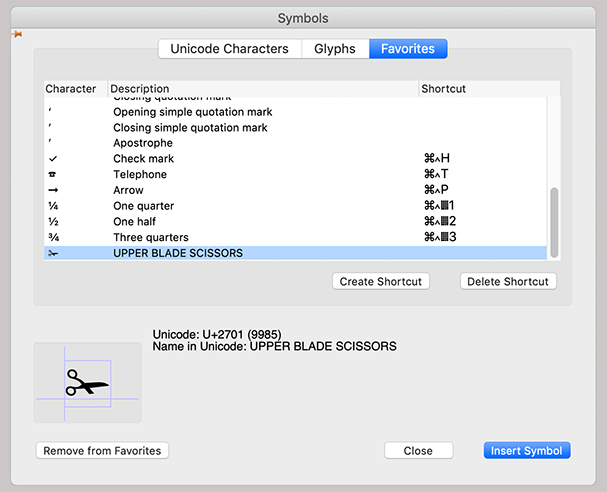
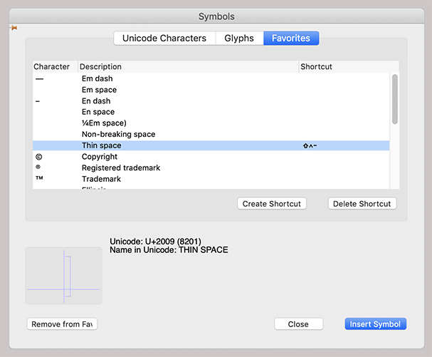
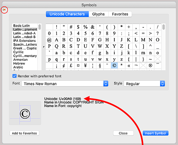
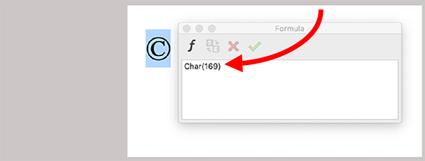
In this panel «Favorites», a series of characters are already listed upon installation. One of them is «Thin space». Anyone who values correct typography will also make this character usable with their own shortcut. Whenever word spaces should be narrower, e.g., in abbreviations or initials of first names (E. A. Hoffmann), the thin space with a keyboard shortcut is quickly available. Another nice side benefit of these symbol panels are the hints on Unicode characters. Every available character has its own Unicode number. RagTime can calculate with these Unicode numbers in the formulas, or access them (see Fig. 2.36 and Fig. 2.37). In the section on working with spreadsheets and addresses, we will come back to that.

Finally, something useful that could be overlooked: The small pin in (Windows)/beneath (Mac) the title bar. If it is horizontal, the window must be closed again before you can continue writing in your text. If the pin is set vertically by selecting, the window can remain open while capturing text, and you can access the symbols, glyphs, and favorites again and again.

Another look at the fonts

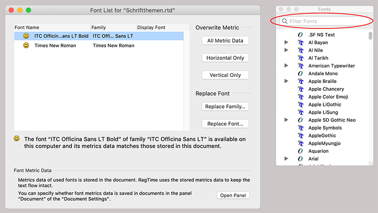
When we are on the topic of special characters, types, and fonts, for the sake of completeness, let's also call up the auxiliary «Fonts List» and the palette «Fonts» (Fig. 2.38). In addition to TrueType and PS Type1 fonts, RagTime now also fully supports OpenType fonts. The «Fonts» palette makes it easy to find the desired font on the computer. Entering some letters limits the list to those fonts whose names contain the entered letter sequence – not necessarily at the beginning of the name.

The «Fonts List» window has a slightly different function. Here you can check whether all fonts used in the document are available on the computer and whether they have the same character spacing and style.

AutoText

Fig. 2.39:

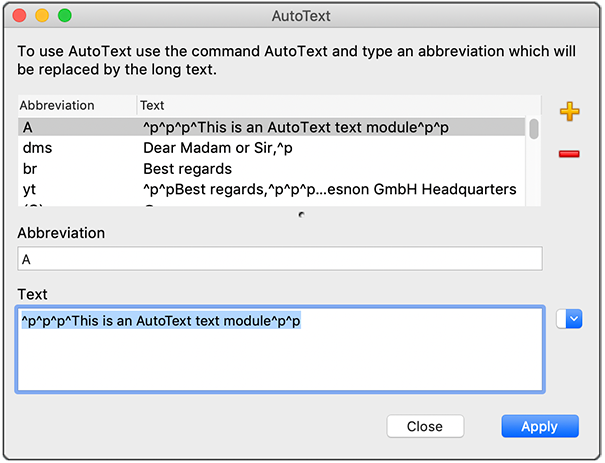
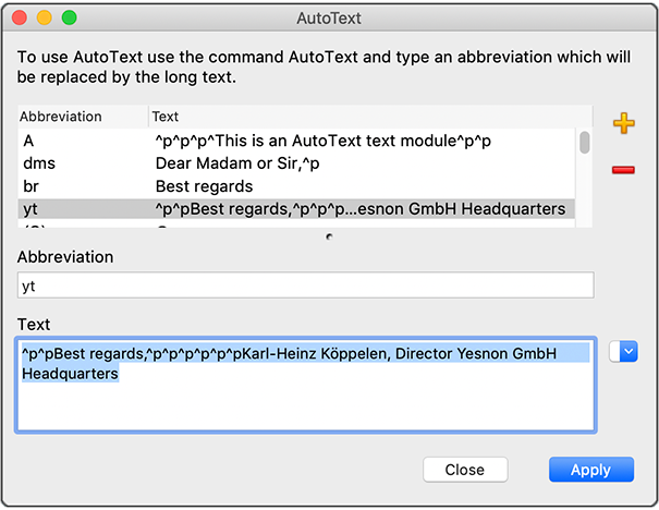
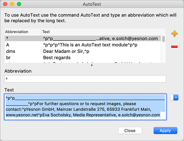
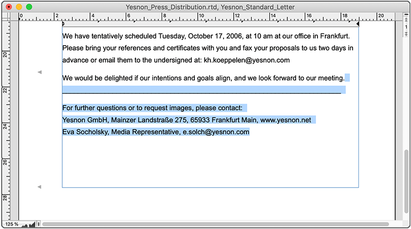
Under «Edit», there are the two functions «AutoText» (A'/c) and «AutoText Settings…» (A“'/6c). If you open the settings, you will see in the AutoText window already a series of characters and text blocks that you can use with the corresponding shortcuts (see Fig. 2.39). More interesting, however, are your own text blocks that you can enter together with a self-chosen shortcut. In the example of our YesNon media mailing, on the one hand, the sender of the director on the letter (see Fig. 2.43) and the footer of the media text with the person responsible for media contacts consist of AutoText blocks (see Fig. 2.44).

Fig. 2.40:

With the minus sign ICON , you can delete existing entries, with the plus sign ICON , insert new ones. A new entry always appears exactly above the one that is currently selected in the list. Unfortunately, the list cannot be sorted or regrouped in order. Write your text in the lower field – paragraph marks can be written right along –, and enter a shortcut. Click on the «Apply» button, and the text is immediately inserted there in your existing text where the insertion mark was. – These shortcuts have no influence on the keyboard shortcuts that are otherwise present on your computer or in RagTime, since they are introduced with a prefix.

Fig. 2.41:

Fig. 2.42:

Fig. 2.43:

Fig. 2.44:

To insert a text block already stored in AutoText into your running text, press A'/c as prefix, an insertion mark appears (Fig. 2.40), then enter your shortcut for the text block. This inserts the requested text, but until confirmation with < or T, it is displayed underlined (Fig. 2.40/2). Simply continue writing in your normal text. The inserted text is now completely independent of the AutoText, i.e. you can edit and format it like a normally entered text (see Fig. 2.40/3&4). The text blocks – these can be individual characters, abbreviations, words, or longer text passages – can be changed in AutoText at any time. However, changes in AutoText will not affect AutoText entries that have already been used in your documents. AutoText can be used everywhere you work with text, regardless of the type of component.

Further in the text with facilitations

In the example of the YesNon language school's media mailing, further special features are worth mentioning. The director's signature was scanned and built in as a flowing picture component in the text. Understandable that our director does not want to sign two hundred letters by hand. The signature will look like the original at first glance on a good PostScript printer. More about flowing picture components can be found in Chapter 3.8 “Flowing elements”.

Fig. 2.45:

What does not stand out in this example is the page break, i.e., the deliberate or automatic page change of the text from the end of one to the beginning of the next page. If containers are connected with a pipeline, the text runs automatically anyway. In our example, it works out exactly with the texts at the page end by chance.

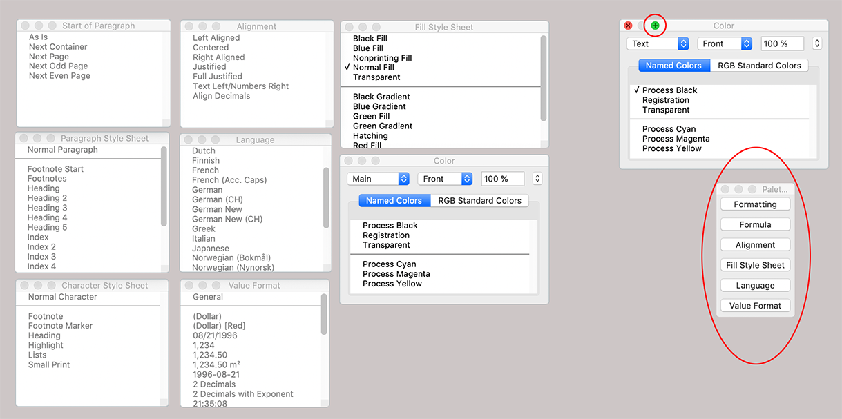
Tip:: For better working and faster access to the individual palettes, there are two aids in RagTime 7: the formatting palette and the palettes dock (Mac only). Many commands and functions are thus directly accessible by mouse click.

But if you want to force a page break at a specific text position, there are three possibilities: You enter so many paragraph breaks until you have your text automatically on the next page, or you reduce the height of the container from below up to the line that should jump to the next page. Of course, this is not possible for layouts that depend on a master layout. The third and actually only correct approach is via the paragraph break; in text mode under «Format ➝ Start of Paragraph». This gives us the opportunity to present another facilitation for working with text.

Tear-off/Dock

RagTime allows tearing off submenus under various pop-up menus. This turns the submenus into palettes that can be kept on the workspace to have permanent and quick access to their functions. Tearing off occurs when you drag the pointer beyond the edge of the menu area with the mouse button pressed (to the right, up, or down). In Fig. 2.45, those tear-off palettes are compiled that are available under the menu «Format». You can change the size and position of the individual palettes.

Only for Mac users, there is additionally the possibility to click the green button in the palette header and thus supply the palette to the «Palettes Dock». This small palette “collects” all palettes docked in this way under their names. A simple click on the name makes the palette pop up again. This comes in quite handy because the workspace is then not always covered by many palettes, but only by those that you really need frequently at the moment. Nevertheless, these palettes remain quickly accessible and do not have to be tediously torn off from the submenu again. The palettes dock can also be placed arbitrarily on the workspace.

Fig. 2.46:

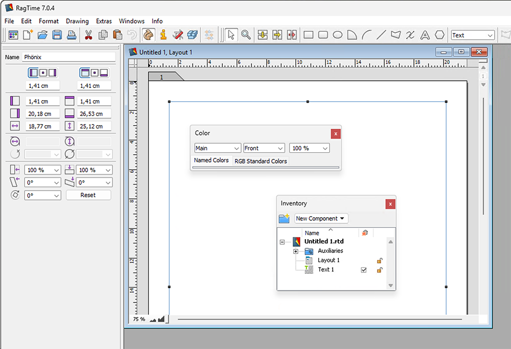
Under Windows, the palettes behave differently: A double-click on the title bar docks them at the window edge, but in full size. Another double-click makes them a freely movable palette again. Palettes can be reduced to a minimal size, little more than the title bar. However, there is no practical palette dock in Windows like there is in Mac. In Fig. 2.46, the object coordinates palette is docked – each palette has its fixed assigned side of the window where it is docked. The Inventory – under Windows also a kind of palette – and the color palette are free-floating, the latter reduced to minimal size.

The formatting palette

It is already explained in detail at the end of Chapter 1 “Order at all levels”. The formatting palette can also be “hidden” in the palettes dock on the Mac. You can call up the formatting palette via the pocket knife symbol ICON in the toolbar. It is a useful work tool, as it allows quick formatting of texts, fonts, colors, and some other settings that you can access faster this way (see Fig. 2.47) because they are united in a single palette instead of having to be laboriously collected. But if you have formatted text with the help of this palette: Do not forget to make a character and/or paragraph style sheet from this formatting! A disadvantage of the formatting palette: if all setting possibilities are open, it covers a large part of the workspace on normal screens. You can remedy this by clicking in the title fields of the individual sectors, whereby the palette becomes correspondingly smaller.

Fig. 2.47:

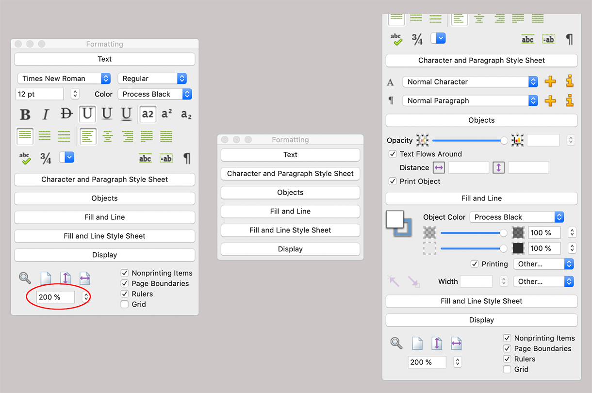
In addition to the actual formattings, the «Display» sector of this palette is particularly interesting. With it, the display size in the current window can be set “steplessly” as desired. There are direct commands to display the whole page in the window, the whole height, or the whole width. The quick showing and hiding of nonprinting items is just as practical as showing and hiding rulers, grids, or the gray displayed page boundaries that are not printable for the connected printer. If the formatting palette claims too much screen space for this comfort, or if the movement of the pointer to the formatting palette seems too cumbersome, there is always the possibility to create own keyboard shortcuts for the desired commands.

“Shortening” the work

We started from the «Paragraph Break» to show some work facilitations that can mainly be used in text mode. For the example «Paragraph Break», the keyboard shortcuts in RagTime are just as practical as for the display commands mentioned in the last section. There are keyboard shortcuts for the most diverse commands and functions.

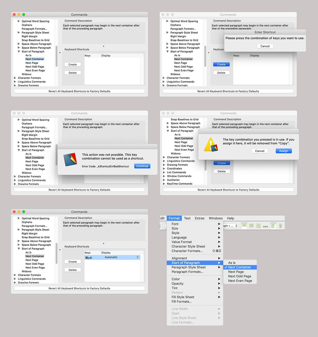
The interesting thing about this is, of course, that you can create your own keyboard shortcuts, especially for those commands that you need most and that might otherwise be difficult to access via drop-down menus or info panels. In the individual selection menus of RagTime, those functions that already have a keyboard shortcut are displayed (see e.g., «Edit ➝ AutoText»). The possibilities for own shortcuts are almost endless – and also unmanageable. Open the corresponding window under «Extras ➝ Keyboard Shortcuts…». The listing on the left with the drop-down switches (triangles) offers several hundred possibilities. Unfortunately, RagTime nowhere knows a clear listing of these «Commands», which often makes finding certain functions/commands very laborious. Especially since the logic of the assignment is not insightful for all functions. At least, when entering letters, RagTime jumps in the list immediately to the command that carries these initial letters. But first, only if really all subgroups are expanded, and second, sometimes you know which command you are looking for, but not exactly how it is named.

Fig. 2.48:

We have compiled all preset commands for you in Appendix B “Keyboard shortcuts” in a list. In addition, we give you recommendations for own keyboard shortcuts in an additional list.

Define keyboard shortcuts

If you have found the searched command in the window «Commands», select it, and press the button «New» under «Keyboard Shortcuts». Now you are prompted to enter a keyboard shortcut: if your desired shortcut is not possible, a warning message appears. Likewise, if your shortcut is already assigned. Then you have the choice to use this existing shortcut new for your command; it no longer applies to the original command from then on. We advise against that. Because who knows – suddenly at the next work exactly this command is important. As soon as you have chosen and entered your shortcut, it also appears in the menus of RagTime. In the example of the forced text break, you can now begin a paragraph that should be in the next container with the shortcut defined by you (in the example according to Fig. 2.48 1AA) and then continue writing immediately without having to use the mouse. The shortcut does not necessarily have to be used at the paragraph beginning. If the insertion mark is somewhere in a paragraph, or a text position in the paragraph or even the whole paragraph is selected: With this shortcut, you always give the command to begin in a new container.

Fig. 2.49:

Fig. 2.50:

Fig. 2.51:

Fig. 2.52:

Everything right – everything good?

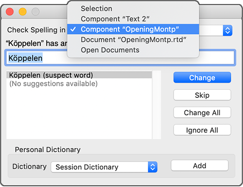
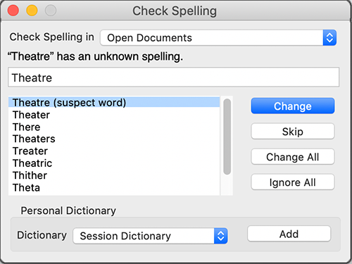
Now the texts for letter and media notice would be finished. But possibly a few errors have still crept in. For that, there is «Extras ➝ Check Spelling…». By the way, this is also a function to which you can assign your own keyboard shortcut if used more frequently.

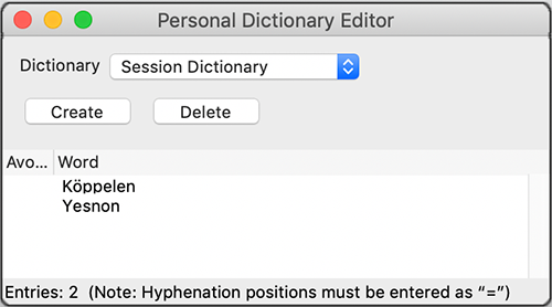
The spell check can refer to a selection, a component, a document, or all open documents. RagTime gives suggestions for unknown words, what might be meant or what is orthographically correct. Also repeating words that are close together are noted (see Fig. 2.49 and Fig. 2.50). The other functions of the spell check explain themselves. What the spell check does not show are hyphenations and, for example, double spaces. The «Check Spelling» window is, of course, linked to your dictionaries. Since RagTime 6, all dictionaries are supplied. Good about RagTime is that you can still create your own dictionaries: For the current correction run a «Session Dictionary», for your company one own (with spellings of your company name and industry terms) and also otherwise for all possible projects one each. These dictionaries do not have to lie in the RagTime folder like the RagTime dictionaries, but can be stored anywhere on your hard drive or on the server.

Fig. 2.53:

Fig. 2.54:

Fig. 2.55:

Fig. 2.56:

Hyphenations: where and why at all?

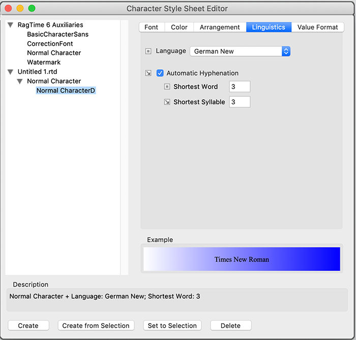
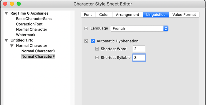
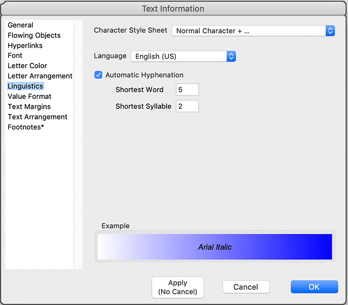
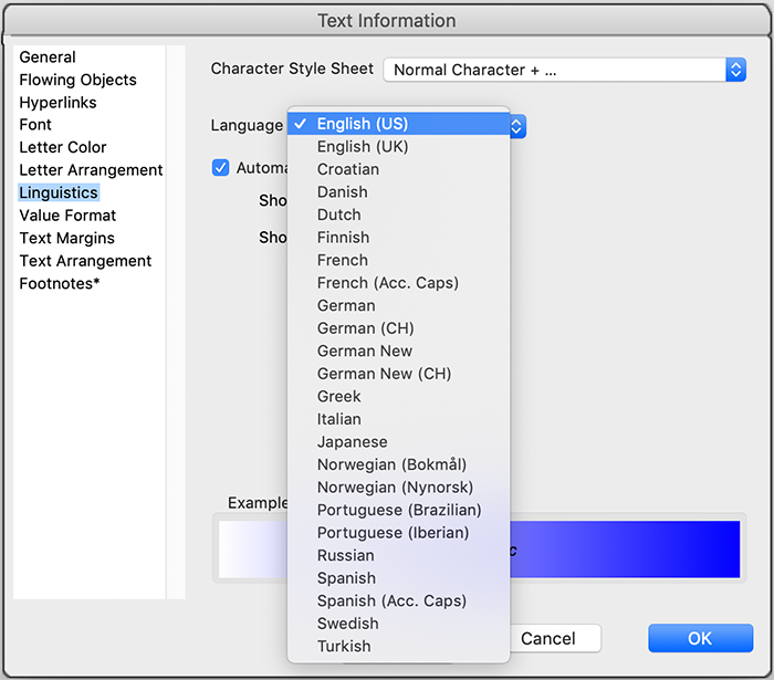
You can specify the conditions under which separations should be inserted in «Text ➝ Information ➝ Linguistics». In this panel (see Fig. 2.55), the hyphenation conditions for the automatic hyphenation can be set, or on the other hand, determine that no hyphenation should occur at all. With RagTime, however, you can influence hyphenations much more specifically: In the panel «Character Style Sheet Editor ➝ Linguistics», an inherited style sheet with a different linguistics can be created for each character style sheet. This means that in a single text, several dictionaries can be queried. Specifically: You assign to the English, French, or other language text parts in your text each an own, inherited character style sheet with the corresponding linguistics (see Fig. 2.53 to Fig. 2.56). Of course, you can also set for each font and language whether you want to suppress hyphenation in general (if «Automatic Hyphenation» is not selected). Under «Format ➝ Language», you can simply check which language or which dictionary is currently being used.

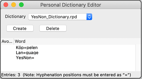
In the dictionaries where you record your new words, hyphenation commands are also possible. Enter «=» between the syllables to be hyphenated (without the quotation marks), so the word is hyphenated exactly there.

Fig. 2.57:

Fig. 2.58:

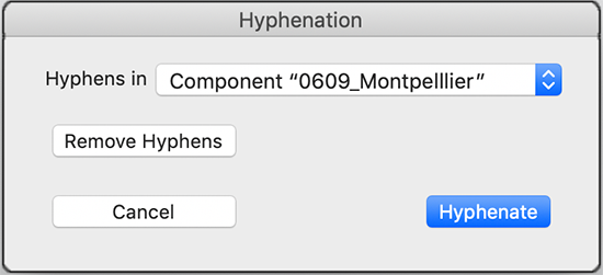
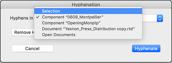
If you append a «=» to the end of a word instead, this word is fundamentally not hyphenated (see Fig. 2.52). Hyphenation is still possible at the end even if you had previously turned off automatic hyphenation: Under «Extras ➝ Hyphenate…», the component can be selected (see Fig. 2.57/Fig. 2.58), in which hyphenations should be made (or also removed). Conversely, if you want to retain hyphenations in imported texts, the setting in the window «Settings ➝ Text» applies.

Search and replace with style

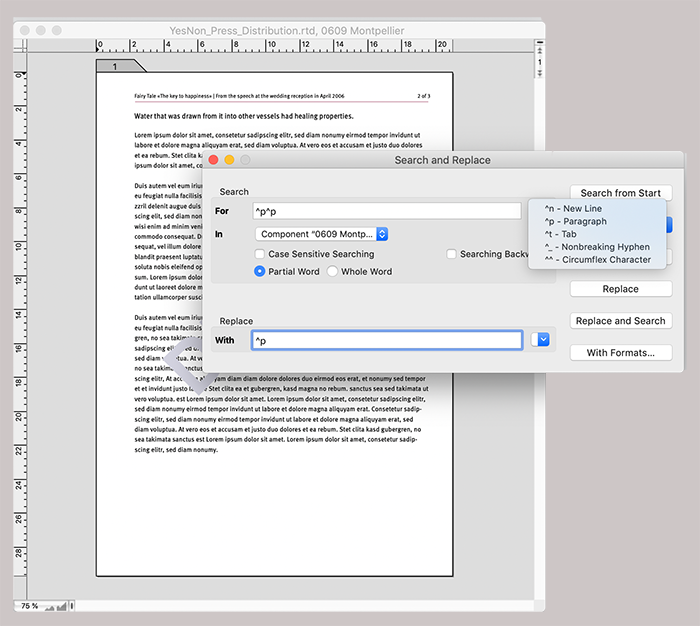
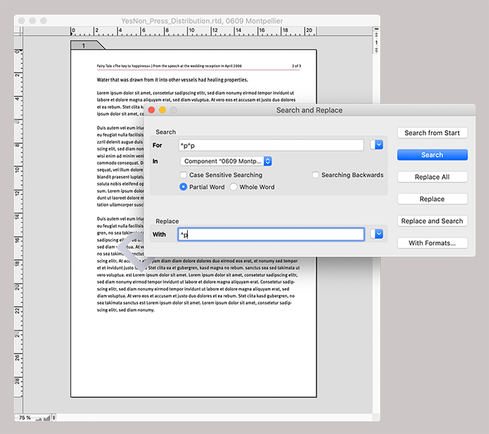
It is obvious that you can enter word parts, words, sentences, sentence parts, etc. with «Edit ➝ Search and Replace…», or AF/6F, and replace them with another text. Eliminating double paragraphs or spaces, removing or adding paragraphs and tabs, replacing normal hyphens with non-breaking hyphens, etc. are all part of the standard repertoire of the search/replace function.

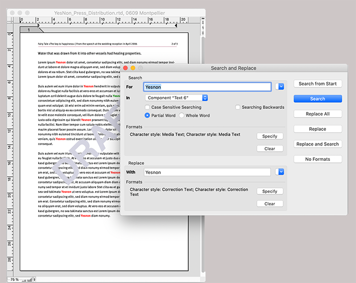
For example, set two spaces above and one space below, so the whole document can be freed from double spaces in one go (see Fig. 2.62). Particularly interesting is the search or replace according to style specifications. This allows you to search text passages according to character style sheets and replace them if necessary (see the example with the red and uppercase written YESNON in Fig. 2.61). When importing texts, a document is often “contaminated” with unwanted fonts, character and paragraph style sheets. There, searching and replacing according to fonts and styles can be a great help.

Search and replace above all

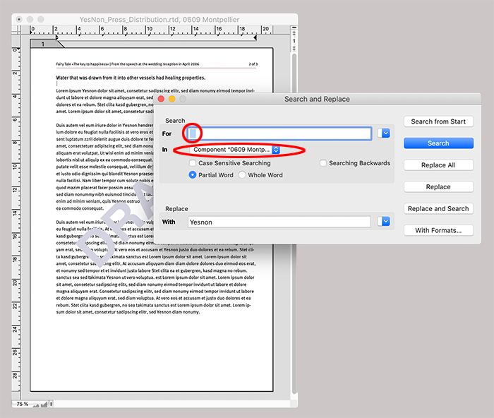
We have presented «Search and Replace» here in connection with our media text. That would suggest that it is a function that can only be used in text components. However, «Search and Replace» in RagTime includes all components that contain text or graphic text, regardless of the component in which it is located. Only buttons are not searched.

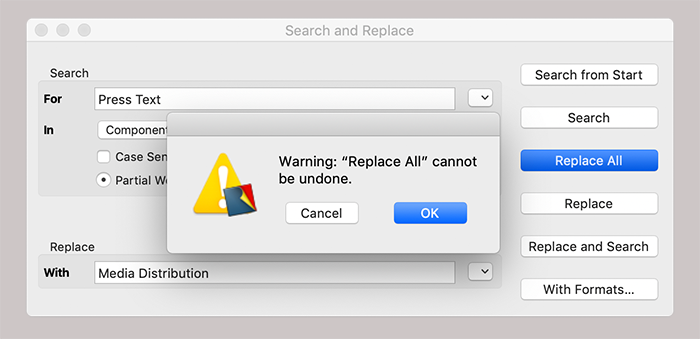
The function can be applied in one pass to a selected text area, an entire component, the entire layout, or even to all open documents (see red marking in Fig. 2.62). But attention: if you intend to press the button «Replace All», then it is important to check once more exactly what is selected under «In». If it says «Open Documents», for example, alarm bells should start ringing! Because the fatal thing is: «Replace All» cannot be undone.

The warning message (see Fig. 2.63) is easily confirmed too quickly in haste – then it has happened and possibly the work of several hours is destroyed.

Fig. 2.59:

Fig. 2.60:

Fig. 2.61:

Fig. 2.62:

Fig. 2.63:

A whole lot of text

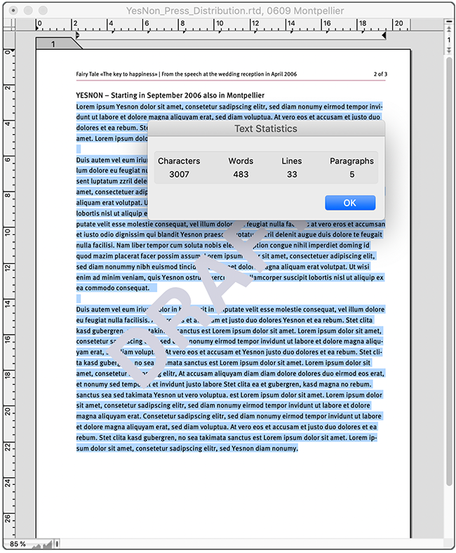
In media reports, or if you have to deliver articles for magazines and books, the desired text amount is usually specified. Then it says, for example: «A maximum of 2500 characters is desired.» In RagTime, you can simply check the text amount in text mode by selecting «Text ➝ Text Statistics…». The text statistics counts all letters, words, lines, and paragraphs in the current container. In the example of the media mailing, letter text and media text are on two pages, but contained in containers connected by a pipeline, thus in a single text component (see Fig. 2.27).

If you do not want to count the whole text, first select the text passages over which you want a text statistics (see Fig. 2.64). Unfortunately, the small panel with the text statistics is not referable, that is, you cannot automatically incorporate the counting results into a text or spreadsheet using a formula. You must write down the information.

The length trick

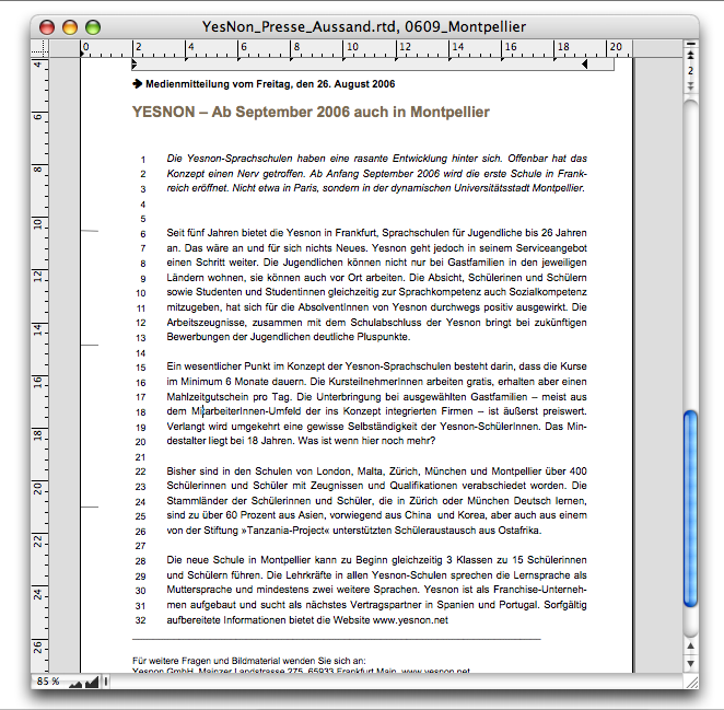
Anyone who frequently deals with media reports can create a good aid. We have created a spreadsheet on our YesNon media report (transparent filling for the cells and for the container). The line spacings in the text are fixed at 16pt – so we have also set the row heights in the spreadsheet to 16pt. Then we entered the formula «Row» in cell B1 and copied the cell down as far as we will roughly need it (e.g., to row 1000). These numbers now indicate the row number and make it easier for a proofreader, editor, or layout designer to work with the text. The spreadsheet can then be dragged to the following pages using pipelines. This “row counter” actually has nothing to do with the exactly counted text amount. For this purpose, we have created a checkbox in cell A3 that allows us to show or hide cells A1 and A2 (see Fig. 2.67).

Fig. 2.64:

Fig. 2.65:

Fig. 2.66:

Fig. 2.67:

Fig. 2.68:

Fig. 2.69:

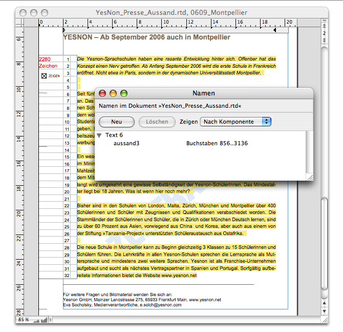
Cell A1 then contains the formula that either inserts the length of the text or simply nothing:

Formula 2.3:

In cell A2, it is only the word «Character» that we want to be either visible or invisible, depending on whether the checkbox in cell A3 is selected or not. Therefore, use the following formula:

Formula 2.4:

Names for calculating

That's nice and all but what is meant by «mailing3» in the first formula? The function «Length» normally returns the number of characters of the referenced cell in a spreadsheet. Here, it refers to a name that we have given to our media text. Just as you can give names to the components in the Inventory, you can also give names to text parts (letters, words, lines, paragraphs, etc.): Select the relevant text and assign a name to the marked text with «Auxiliaries ➝ Name Editor ➝ Create» (see Fig. 2.66). The first characters of the selected text appear on the left side of the window, and on the right side, the letters – from to – that belong to this text component are displayed. Now you can still insert a meaningful name on the left (in the example «mailing3») and close the window. This makes your text “calculable”. If you do not want the information in cells A1 and A2 to be printed, you can select the «On Screen» option for these cells under «Spreadsheet Information ➝ Cell Contents ➝ Visibility» – This allows you to do the opposite of what you would normally do, i.e., not refer to the text from spreadsheets, but use parts of the text with their names in formulas. If you have referenced such a text in a spreadsheet cell – via an assigned name – it can even be accessed from there in other documents – this is not possible directly. And what is the whole thing for? – Whenever you change something within the text passage that has been labeled with the name, all references are automatically adjusted. The same thing happens as with text calculated from spreadsheet cells. Consequently, the font settings can also be transferred: With a hash mark «#» before the name, e.g., «#paragraph5» if the name was «paragraph5», you will see the named and referenced text passage with the same font, size, and color.

And again something for the archive

Transfer a spreadsheet component such as the one we have just created directly into the form or the master layout of your media texts. If you only need such a counting aid occasionally, give the spreadsheet a name (e.g., «Text Counter») and push this into a new document for components and objects worth archiving. Of course, you must update the reference with the name you created in another text document and assign a name for the “text count passage” there.

Fig. 2.70:

Last corrections with equalizing

Before sending, perhaps as the last “correction aid” for the almost finished layout, let's take a quick look at the function «Drawing ➝ Equalize Objects». This function works on the same principle as «Search/Replace». So it needs characteristics that belong to the first or original object so that it can be found by RagTime at all.

Tip:: Equalizing objects belongs to those functions that have been in RagTime for a long time. So nothing new for experienced users. As in other functions of RagTime, there are also a few special features hidden here that are quickly forgotten if not used daily.

Then, you need to define those characteristics that you want to transfer to the other objects. In many cases, however, it is simply a matter of creating a new object and copying it to all other pages using «Equalizing».

Fig. 2.71:

Fig. 2.72:

Fig. 2.73:

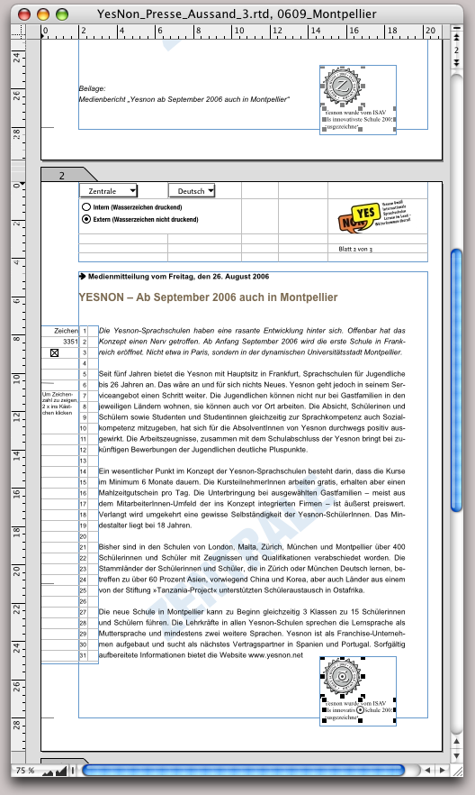
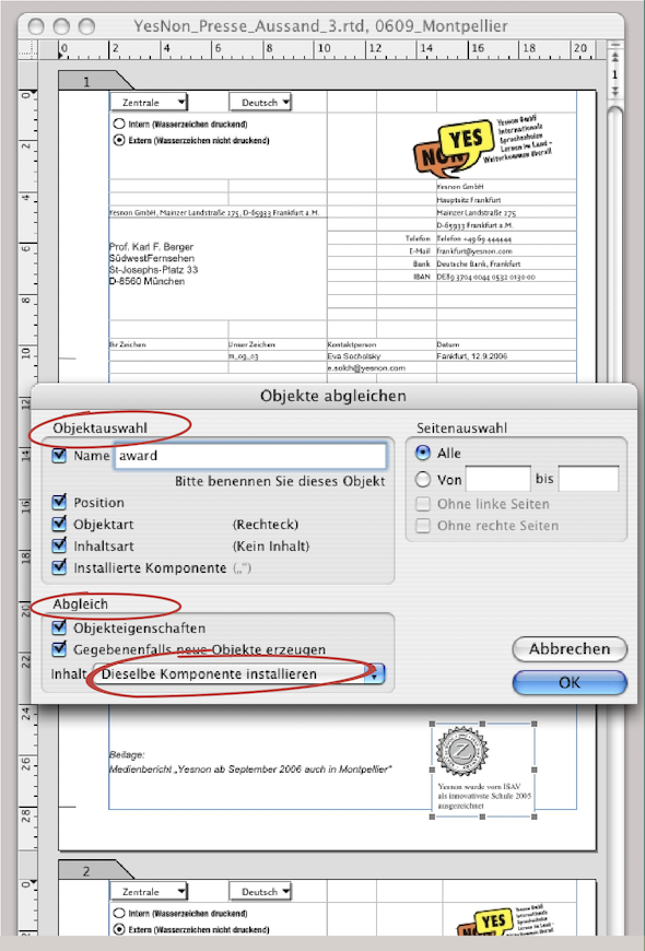
In our example of the media mailing, the case has occurred that the YesNon school has just been awarded a prize. This emblem should also appear on the media text. So, on one page – it doesn't matter whether it's the first, last, or any other page – we imported the emblem as an EPS file in an image component. Underneath, we wrote the explanation using graphic text. Picture component and graphic text are integrated into a drawing component (see Fig. 2.70 and Fig. 2.71). The advantage of a drawing component is clear: each object can be moved and modified individually, and the corresponding objects on the other pages are moved or modified without having to perform another «Equalize Objects» operation. However, this only applies if «Install the same component» was selected during the first object equalization.

Fig. 2.74:

Almost like search and replace

The principle of equalization: The options under «Object Selection» help RagTime to identify the object to be equalized. The options under «Actions» and «Page Selection» give the parameters how and where the object should be newly installed or changed. As soon as the object to be equalized has a name, it is identifiable. However, a small trick can lead to problems. Therefore, we have solved the same task as in the previous example here with two separate components: With a picture component and a graphic text – thus without both being “packed” in a drawing container. If an object is moved during object equalization and you want the same objects on the other page to also be at this position on the page, then under «Object Selection», «Position» must not be selected under any circumstances.

Fig. 2.75:

RagTime then searches for the objects that are at the same position as the selected object. Nothing is found, which is indicated by a message (see Fig. 2.76). By the way, the reason why our example only mentions two pages in the warning and confirmation messages is because our document only has three pages. In such an equalization, only the name may be selected so that it works. In this way, the size and position of the emblem have been equalized in Fig. 2.73 and Fig. 2.74, as have the position and font color of the graphic text.

To conclude this brief excursion into the functions of object equalization, here is a rather cynical remark: do you remember that we originally built the example document on a master layout? And there – that is only logical – «Equalize Objects» doesn't work anyway (see Fig. 2.75). So we could have simply added our award notice to the master layout… However, we deliberately detached the document from the master layout just to demonstrate the principle of object equalization.

Undo the equalization?

Equalizing objects cannot be undone. This is a minor disadvantage among many advantages: once installed, the objects created in this way cannot be easily removed. Of course, the newly created objects can be deleted from the Inventory. This leaves an empty frame everywhere in the layout. It is not visible in the printout, and if these frames do not interfere with the layout, you can leave them where they are.

Fig. 2.76:

It's different with graphic text. Graphic text is known not to be listed in the Inventory. So you would have to laboriously delete these objects individually on each page again. But there is a trick there too: assign the transparent color to the text to be deleted on one of the layout pages and then perform an equalization. The graphic text objects are still on the pages afterwards, but no longer visible. Instead of «Transparency», you can also delete the text down to a single space and then perform the object equalization.

Fig. 2.77:

2.5 Addresses as share capital

Addresses are an important component for every company when it comes to smooth administration and successful acquisition. Address files are something of an everyday occurrence, especially for small and medium-sized businesses, but if the data is poorly prepared, they can also be a huge time waster. In our “school example”, we first assume that we need an address file for our media mailing. Using a spreadsheet, we play through various situations that make working with addresses difficult – and where RagTime can help out of the jam.

2.5.1 The file with header and planes

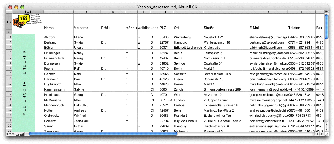
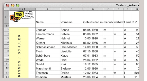
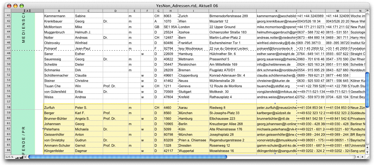
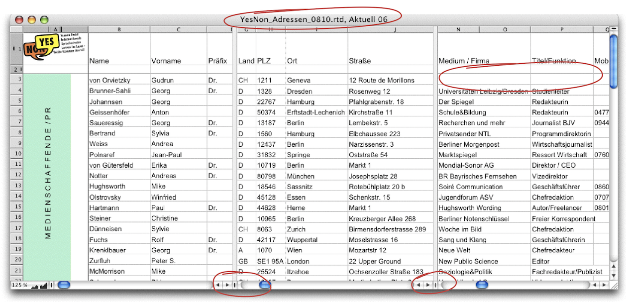
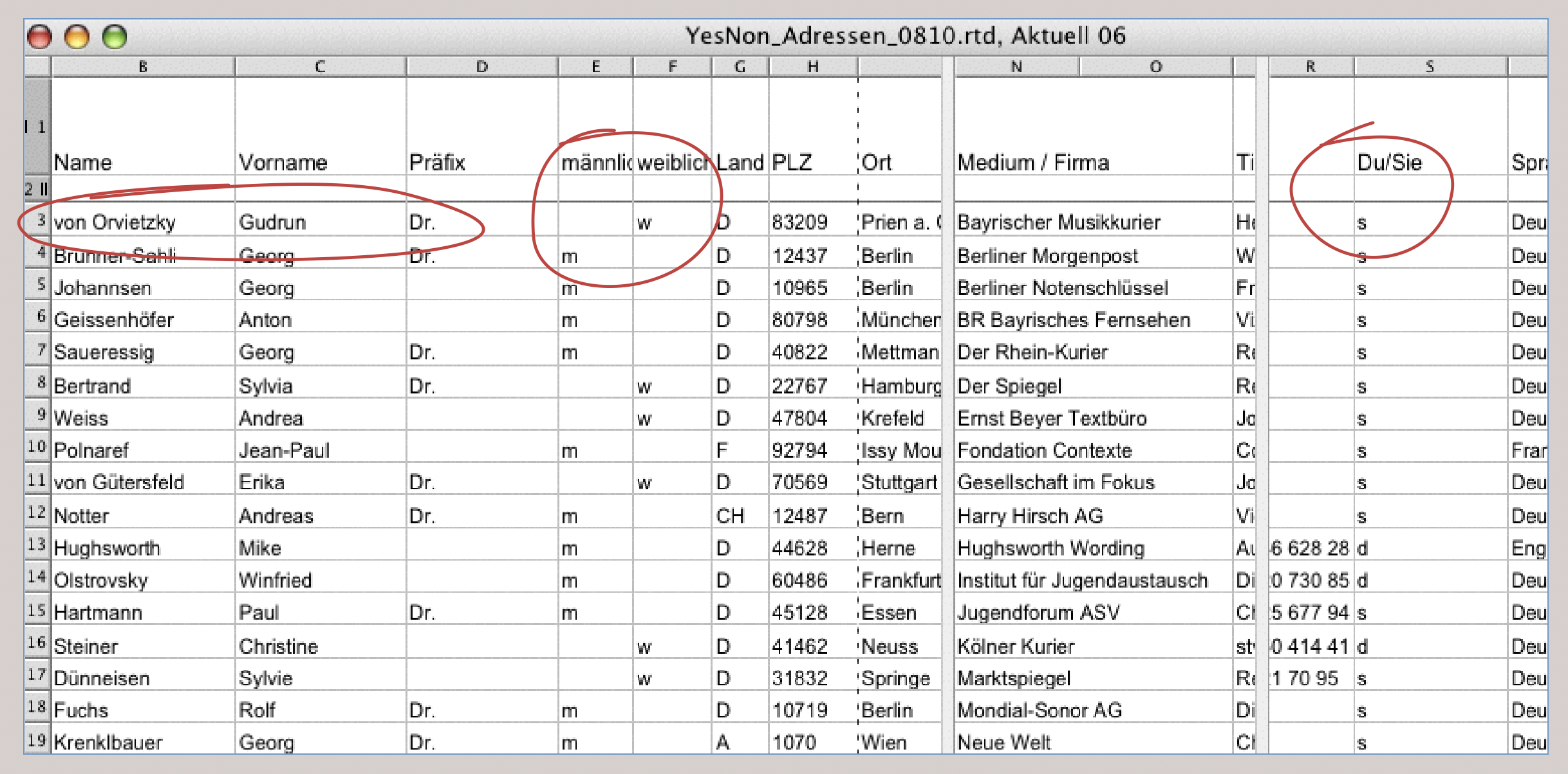
Fig. 2.77 shows a spreadsheet in which the respective address groups are contained in different planes. Plane 1 contains all internal addresses of the YesNon schools, plane 2 all students, plane 3 all partner companies, and plane 4 contains the public relations addresses with the journalists and media professionals. The spreadsheet is designed with headers (title rows) and margin column (title column).

Headers are always advantageous when the spreadsheet contains so many rows that it is distributed over several pages in the layout. Then the header automatically appears on every page. In the example of the YesNon address list, the header also contains the logo in cell A1. Column 1, on the other hand, is used as a labeling column. Here, color fields and text labels on each layer make the address groups immediately visible. This form of address management also has its advantages and disadvantages. The advantage is that all addresses are accommodated in a single spreadsheet. The disadvantage: in all layouts, the column widths (and row heights) are exactly the same width or height. You can change the title designations (cf. Fig. 2.78 and Fig. 2.80), and the cells can be defined individually (components, unions, fill style sheets, character style sheets, etc.) but the grid of the spreadsheet changes on all planes if you change column width or row height in one plane.

Even more essential: if you delete entire columns or rows, it also deletes the relevant columns or rows in all other planes. This means that you can only make changes within cells or cell ranges. It is therefore a matter of personal preference whether you prefer to create a separate spreadsheet or even a separate document for each target group. And finally, you can also accommodate all addresses in a single spreadsheet and a single plane. Then you will probably assign your own code for each address group in a column to be able to access it in mail merges. Regardless of how you organize yourself, the topic of headers or title columns is interesting regardless.

Fig. 2.78:

Fig. 2.79:

Fig. 2.80:

Fig. 2.81:

Fig. 2.82:

Headers as desired…

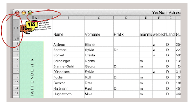
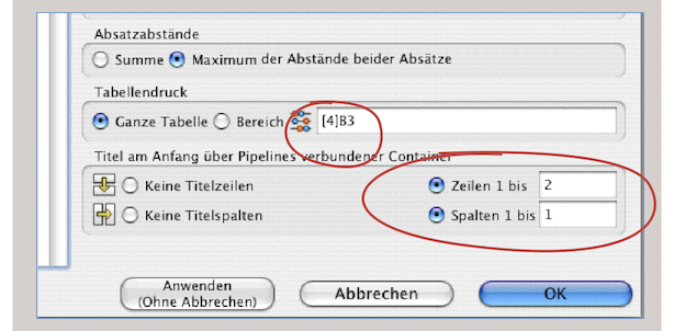
In Fig. 2.78, column A and rows 1 and 2 are specially marked. So you immediately see whether and how many rows or columns are reserved as title row or title column. The setting for this is simple: Call up the spreadsheet information and there under «General ➝ Titles at the Beginning of Pipelined Containers» enter the desired row or column number on the right (see Fig. 2.79). If you change the relevant number, the corresponding option is automatically activated. If the value is left at 1, you have to do it yourself. That we are here in plane 4 (red circle) has no influence. The entry of the title rows and title columns can be made independently of the displayed plane, but: it always applies to all planes. In Fig. 2.80, plane 2 with the addresses of the students is visible. Title rows and title column are the same as in plane 4 (Fig. 2.78).

…and pipelines as desired

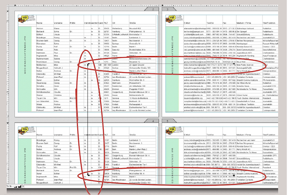
How these title rows and title columns take effect becomes clear in Fig. 2.81. On a double-sided layout, the container of the left page was connected to that of the right page via a horizontal pipeline. The container of the left page was also connected to the container on the left following page – and this in turn to the one on the adjacent right page. Title rows (or title columns) are repeated on all pages, while the continuation of the spreadsheet is displayed afterwards.

Fig. 2.83:

Fig. 2.84:

Fig. 2.85:

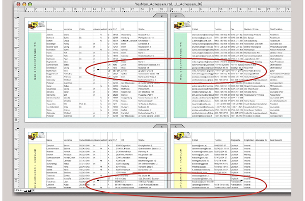
In the example in Fig. 2.82, the containers of the left and right page were also connected with a horizontal pipeline on the lower double page. Then the same spreadsheet with the addresses was dragged from the Inventory into the left container and then plane 2 selected. This way, you can also display all planes (address groups) one below the other in the layout.

2.5.2 Import addresses

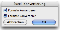
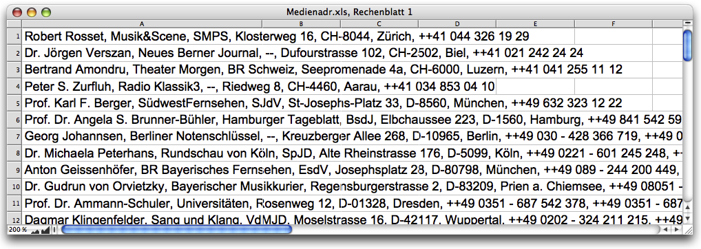
In our exercise, we now continue to assume that the managing director of our school in Munich has sent us a file with interesting addresses of media professionals. He has emailed us an Excel file «Mediaadr.xls.». Upon importing, the usual message appears (Fig. 2.83). But then a rather annoying picture emerges (Fig. 2.84) because the data is written consecutively per row. However, we need it separated. Poorly formatted addresses are a recurring problem. Fortunately, there is still some consistency here, as the individual address components after the name are all separated by commas and spaces. For sorting into columns in our address file, we need a tabulator as a separator between the individual address components.

2.5.3 Three ways to good entries

The simplest way: Open next to the address list (Fig. 2.84) a new layout and select the command «Windows ➝ Tile Windows Vertically».

Fig. 2.86:

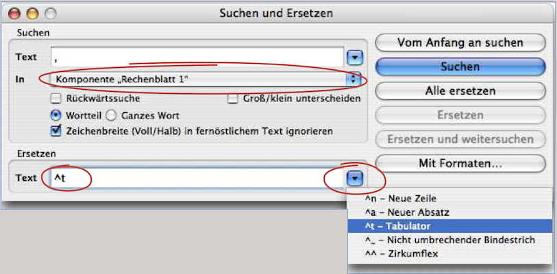
Select all address entries in the spreadsheet, copy the entries, and paste them into the text frame in the layout. Now you can use «Search and Replace» to find the comma followed by a space and replace it with a tab character using «Replace All» (see Fig. 2.85). However, please ensure that the newly created layout or text component is selected in the component selection (marked with an elongated circle), rather than the spreadsheet.

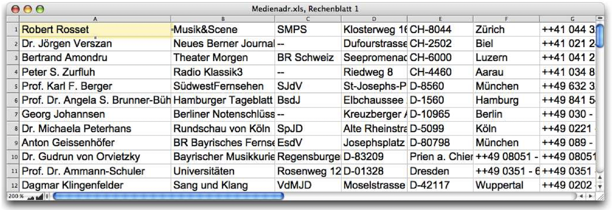
Bring the modified data back into the address file: «Select All», (in the text frame), «Copy» and then «Paste» into the first cell (A1) of the spreadsheet. The spreadsheet with the modified entries should then look like Fig. 2.86. Certain entries – circled – must then be edited manually by copying or dragging the cells to the correct location or moving them to the correct location using «Spreadsheet ➝ Insert Cells».

2.5.4 Formulas for correction

Anyone who has to edit a lot of addresses looks for simpler, automated processes that require as little manual post-processing as possible. Using the example of the re-imported addresses, which still do not fit our address file, we show two such solutions.

Column A contains first names, last names, and prefixes (i.e., Dr. or Prof. or both) all in a single cell. However, as shown in Fig. 2.2 and Fig. 2.12, we want to have these three parts in separate columns. Before performing such tasks or entering special formulas, it is best to make a backup copy of the file under a different name so that you can revert to the original data if necessary. We will now continue working with the newly saved file under the name «Addresses_Converter». The first solution we show looks a little complicated, but it is intended to make the function of the formulas clearer. The second is the more elegant solution, with vertical search. It seems like mysterious magic (at first glance). Those who are more familiar with the formula functions «VSearch» or «HSearch» («V» for «vertical», «H» for «horizontal») will quickly realize their versatility.

2.5.5 «Mid» & «Length» in formulas

The functions «Mid» and «Length» refer, just like «Right» and «Left», to texts. This allows word parts or individual characters to be extracted from them and used as “text modules” for other cell contents. In our case, we use them in formulas to automatically separate prefix, first names, and last names.

Fig. 2.87:

First, insert six additional columns to the right of column A in the newly created spreadsheet «Addresses_Converter» («Spreadsheet ➝ Insert Columns»). As the first step in entering the formula, we search the cells in column A for the prefix, i.e., «Dr.»/«Prof.»/«Prof. Dr.» etc. Since we are searching for clear text segments here, it is important to know all the spellings that occur in this context (for example, an addition such as «Dr. h.c.»).

A few formula steps

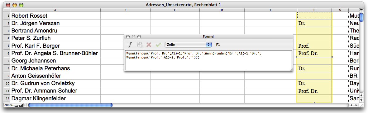
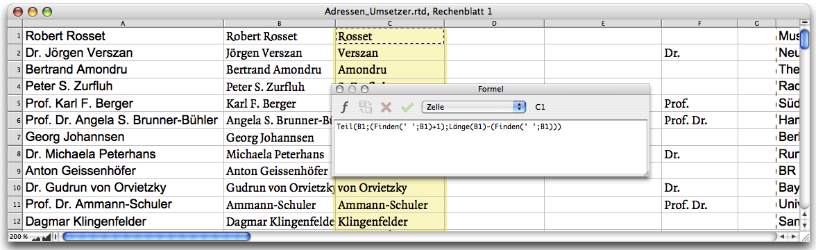
In chapter “Formulas Part 1: And it works”, you got an overview of the functions and formulas. Here we'll continue with practical applications. With the first formula, which you place in cell F1, you ensure that the prefix appears in this cell, provided that one is present in cell A1. Otherwise, the cell remains empty. Of course, this requires a formula with an «If» function. Since different texts are possible, RagTime must find all versions that occur. This can be solved by stringing together several «If» functions. We therefore have to enter our formula as Formula 2.5.

Formula 2.5:

RagTime now always inserts the prefix found in cell A1 into cell F1. If none is found, cell F1 remains empty. «If» functions can therefore be nested as desired. Separated by a «;», this results in a new condition each time, until the “then condition” follows at the end after the last «;». Here, this is called «' '», which means that RagTime leaves the contents of the cell untouched.

«Find» is also a function that requires at least two arguments separated by a semicolon: the text to be searched for and the cell or range in which to search. Like any text in a formula, the search text must be enclosed in single quotation marks, for example 'Prof. Dr.'.

Formula 2.6:

Now copy Formula 2.5, which you entered in cell F1, down column F as far as there is an entry in column A in the same row. In the next step, we refer to the entries obtained in this way in the cells of column F. Enter Formula 2.6 in cell B1. The logic behind this is that if cell C1 is empty, RagTime should simply copy the content of cell A1.

Fig. 2.88:

Fig. 2.89:

If not, it should calculate the length of the cell content F1 (that is the number of characters of the extracted prefix) and then ignore this number of characters at the beginning of the text in cell A1. With «+2», the space between prefix and name is skipped. Strictly speaking, RagTime thus calculates the position of the first character after the space, i.e., the first letter of the first name. The function «Mid» always refers to texts in a cell. After the parenthesis, the cell reference is entered, then (separated by a semicolon) the position of the first character and (also separated by a semicolon) the number of characters to be taken from the text.

Since we can assume in our example that there are no name entries with more than 1000 characters, we choose 1000 for simplicity. By the way, if there is a number in a cell referenced with a text function like «Mid», this number is also treated like text. So a part of this number is detached and taken over. That seems tempting at first glance for certain applications. But attention: if the number changes by one or more digits (e.g., because it is based on an addition formula) it can lead to unwanted partial texts. After copying the formula from cell B1 into the cells below in column B, you will see the first and last names without any prefixes. Now you also want to separate the first and last names. Since we have different versions of the first names – with or without a middle name or its initials – we will take an intermediate step to keep the formulas from becoming too complex. Therefore, enter the following formula:

Formula 2.7:

RagTime should fetch a «Mid» from cell B1. This part is the one that begins after the first space and could have 1000 characters. What remains is the last name, or where an initial stands, also this. This could also be incorporated into the above formula using an «If» function. To illustrate the principle behind the formulas, we have made it more cumbersome by using the same formula principle again in column D. The entered formula in D1 would logically have to be the same as in C1, but with the reference to cell C1.

Fig. 2.90:

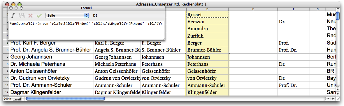
However, here in row 10 there is still this «Gudrun von Orvietzky» (see Fig. 2.88). To keep this «von» correctly with the last name, another «If» function is needed. So enter Formula 2.8 in cell D1.

Thus, for all names with a «von», the cell from column C is fetched unchanged into column D (4 characters counted from the first letter on the left must correspond to the word «von » including spaces). Where this is not the case, the entire part after the space is taken from the C cells. As with all other steps in RagTime, you know from experience: Every few minutes of work or after an important entry, press AS/6S to save the open document.

Formula 2.8:

The last formula entry

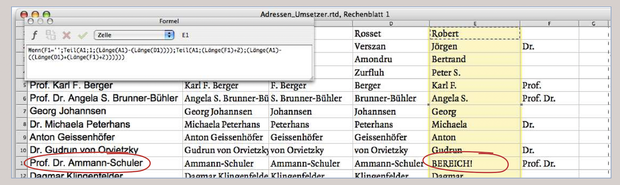
Now all that remains is to filter out the first name(s). This is done as follows: the entries in column A minus the last names in column D and the prefix in column F give the first name. So enter Formula 2.9 in cell E1.

Formula 2.9:

If cell F1 is empty, RagTime extracts the number of characters from cell A1 minus the number of characters from cell D1 (starting with the first character in cell A1). If the cell in column F has an entry, RagTime first determines the correct position in cell A1, i.e., the first character, to start transferring the calculated number of characters. This is determined by the number of characters in cell F1. In the example of «Dr. Gudrun von Orvietzky» this is the fifth character. Now copy cell E1 again into all other cells in column E, provided there is an entry in column A. In cell E11, you will receive an error message saying «RANGE!».

Fig. 2.91:

Fig. 2.92:

RagTime cannot perform a calculation. In this case, it is immediately apparent why: there is no first name in cell A1. You will probably have to obtain this missing first name from the YesNon school in Munich…

Finally a cleaned-up list

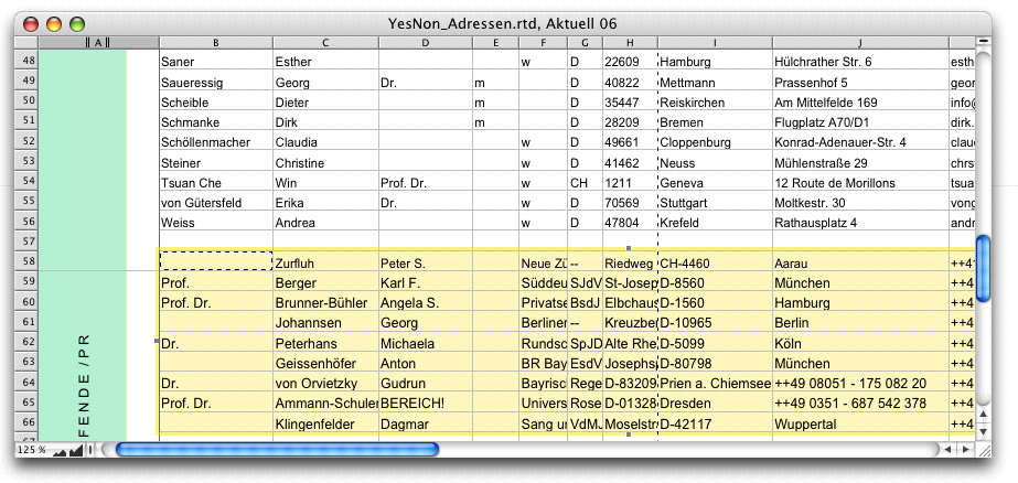
What is now still to do: copy all cells that have an entry from D1 to the bottom cell F and insert this copied range again with «Edit ➝ Paste Special» into the overall list of media addresses (see Fig. 2.91). The checkmark for «Paste Formulas» must not be selected.

Now move the columns of the spreadsheet so that the entries for the new addresses match the order of the existing media addresses in the document (see Fig. 2.92). You can now sort the entries by last name or other criteria.

The same in an elegant way

The same end result can be achieved much more elegantly using the «VSearch» function. This is discussed in detail in “Formulas Part 3: In full swing”. Almost all formula applications that involve copying formulas down a column can be solved with «VSearch». Anyone who works with such problems a lot will be happy to take the time to learn about the formula constructions in chapter “Formulas Part 3: In full swing”, which at first may seem a little complex.

Some more tricks for avoiding errors

In addition to splitting addresses, as described in the previous sections, there are various formulas and tricks for correcting poorly formatted address files in order to prepare the data for use with RagTime 7. Of course, a complex formula construction is only worthwhile if there are many addresses that cannot or should not to be corrected manually. But why not provide a “correction set” of formulas that can be called up and applied as needed? This can also be done very conveniently in the form of buttons. Here, we will only explain the respective principle using individual formulas.

Fig. 2.93:

Fig. 2.94:

Fig. 2.95:

Fig. 2.96:

Fig. 2.97:

Swap uppercase, search spaces

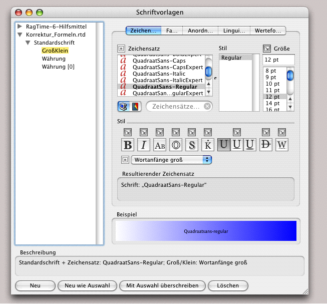
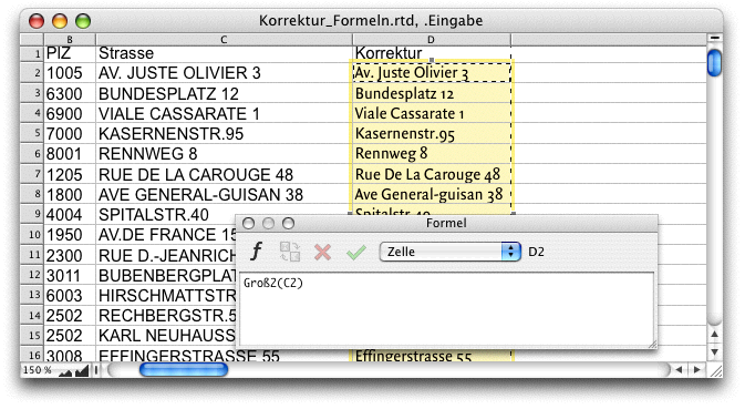
In the example (Fig. 2.94 to Fig. 2.97), all addresses are written in uppercase letters, and in some cases there are no spaces between the street name and the house number. There are two options for capitalization. The first: select all cells and create a new inherited style sheet for your font (usually the standard font) under «Windows ➝ Auxiliaries ➝ Character Style Sheet Editor». Here, simply change to «Upper Case Initials» (Fig. 2.93) and assign this font style sheet to the corresponding cells in the document. All initial letters of each word are now uppercase, and all other characters will be lowercase. Note that the cell content remains unchanged! However, everything will appear as desired on the screen and in print. The same effect can also be achieved with a formula (see Fig. 2.94).

Formula 2.10:

The Formula 2.10 must, of course, be copied down in the spreadsheet, from the first used cell to the last row that has an entry. In Fig. 2.95, we have combined this formula to get the space between street and house number right at the same time. However, Formula 2.11 leads to error messages.

Formula 2.11:

Formula 2.12:

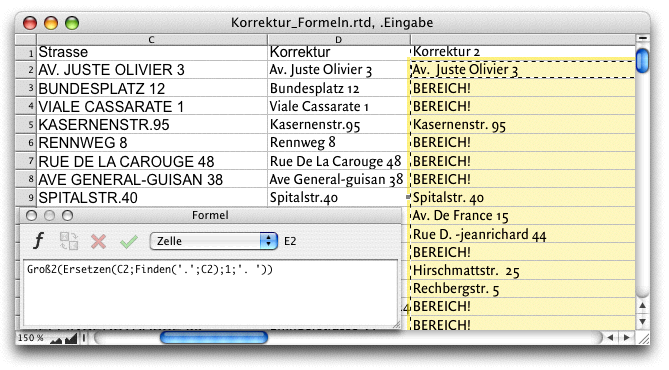
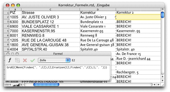
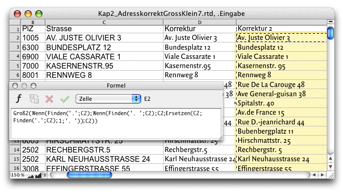
The function of «Proper» is still clear. But then the dot «.» must be found in cell C2 – or the other cells in column C) – (the «1» stands for 1 character) and replaced by a dot with an additional space («. »). Wherever there no dot in column C, nothing will be found, of course, which leads to the error message «RANGE!». So an if-then condition is needed. But even Formula 2.12 is not quite complete yet. RagTime searches in the cells in column C for a dot with a space. If it finds this character combination nothing happens; otherwise it replaces the dot found with an additional space (still with upper and lower case letters). Here, too, there are stille a number of exceptions. As a result, the formula becomes even more complex:

Formula 2.13:

Now all cells that correctly contain a dot followed by a space are transferred (with upper and lower case letters), as are the cells in which no dot is found. In all other cells, the dot is searched for and replaced by a dot followed by a space (see Fig. 2.97). However, if you look closely at Fig. 2.97, you will notice that there are still entries in the corrected column E that are not correct. In the upper and lower case spelling of French street names or in the correct spelling of «Karl-Neuhaus-Straße» etc. Our short section on correction options with formulas should merely encourage you to take a closer look at formulas and formula combinations. In short: if you have a lot of address corrections to do, formula functions such as «Proper», «Lower Case», «Replace», «Find», «Left», «Right», «Mid» in conjunction with «If» combinations can save you a lot of work.

2.5.6 Mail merge with selection

We assume that our address list is correct, as is our letter. How a normal mail merge works – with drag and drop from the address spreadsheet to the letter address – is already described in the «RagTime Training Manual». In the YesNon school example, we therefore want to focus on situations involving deviations or a precisely defined selection from the address file. The operator «&&» has proven useful when entering formulas so that text from different columns can be linked with a space in mail merges. It has the advantage that no double spaces are created if a cell in the spreadsheet is empty. The situation is different if an address element that normally appears on its own line is missing. It looks unattractive if lines remain empty in the middle of the address (see Fig. 2.100). A function similar to «&&» is needed here, and this is called «SmartConcat». Incidentally, in Fig. 2.98, the spreadsheet has been divided so that only those columns that are needed for the mail merge address in the media mailing are visible. You can divide a spreadsheet more than eight times horizontally and vertically in this way if it makes sense for more efficient work.

Fig. 2.98:

Formula 2.14:

Concatenate until the cows come home

The «SmartConcat» function allows for various combinations. However, the formulas then become somewhat more complex, and in some cases even very nested. In combination with the «Char» function, you can specify that the same character is always inserted between the connected text elements – in our case «Char(13)», which corresponds to the end of a paragraph (</T). If the «Normal Paragraph» paragraph style sheet is defined with multiline spacing at the end,

Formula 2.15:

«Char(11)» (=line break) could also be useful. Unicode characters (or other encodings) can be selected with «Char».

Tip:: In these sections, we devote ourselves to the topic of mail merge. The simple drag & drop method is described in the «RagTime Training Manual». Here, we will deal with special applications. The formulas some of which may appear complex, can be archived and will prove useful time and again.

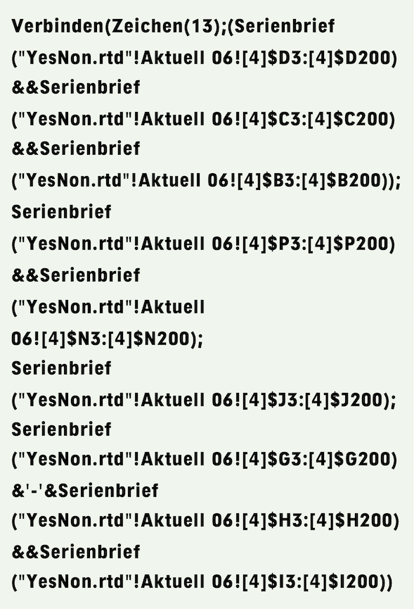
This function is particularly useful when a formula requires text characters that would terminate the formula entry if entered “in plain text”. The Unicode characters and their numbers can be found in the «Symbols» palette. For the mail merge formula, precede the «SmartConcat» function and separate the parts with a semicolon. The mail merge addresses in Fig. 2.99 and Fig. 2.100 could therefore be based on Formula 2.15. «SmartConcat(Char(13))» automatically inserts a paragraph break after each address line. If there is no entry in the corresponding cell of the selected column, the column is skipped. This means that no unnecessary blank rows are created, regardless of whether a street name or job title is missing.

Fig. 2.99:

Fig. 2.100:

The relatively long formula is due to the fact that the reference address to the spreadsheet is already very long: first the document name, then the name of the spreadsheet, finally the plane of the spreadsheet in square brackets, and finally the cells. Since our spreadsheet has a header, the mail merges only start at row 3. The end number 200 should correspond to the number of addresses. And don't forget: the closing last parenthesis!

Another basic point: the mail merge function can be used as such anywhere in formulas. However, multi-line addresses can only be calculated in text components, spreadsheet cells with the content type «Multiline Text» and in graphic texts. The united cells (A6:B13) in the YesNon letter form were given the content type «Text». The content type «Multiline Text» could just as easily have been selected for the united cells. – If you are dealing with text containers outside of a spreadsheet, it is advisable not to place them in the same container as the rest of the letter text, but to create a separate container for them. Pipelines from and to the address field frame are also not very useful.

SmartConcat with &&

The YesNon address file is highly fragmented. This means that we have the prefix, the country, the postal code, the city, etc.

However, we certainly cannot reproduce every entry in the columns on a separate line in the address. That is why – and keen observers will already have noticed this – Formula 2.15 does not calculate correct addresses from the YesNon files. The address elements that belong together on one line are therefore connected with«&&». However, this does not prevent you from starting the entire formula with «SmartConcat(Char(13)» in order to take advantage of the blank line suppression described above. The correct formula must therefore look like Formula 2.16. However, we have shortened the name of the reference file here for space reasons. If you want to reproduce the YesNon example 1:1, you must use the spreadsheet names as in Formula 2.15.

Formula 2.16:

2.5.7 Mail merge for browsing

Once the mail merge commands are started, the whole thing runs automatically. It is therefore recommended to make a test print of a few copies to see if everything is correct. The letters can also be viewed using a print preview. However, this is a rather tedious detour to check the display for each occurrence or the selected addresses. Neither of these checking methods is satisfactory. Therefore, we show here a way that makes it possible to view the letters, or the addresses, as desired and check them before printing. For this, the function «PrintCycle» is used. On the one hand, it can be used to suppress the header when printing, on the other hand, its use allows you to scroll through form letters, and finally, it can also be useful for creating labels with form addresses, as we will show a little later.

Setting up a “Control Center”

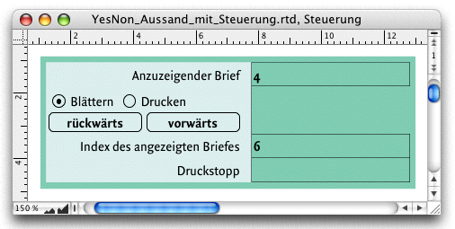
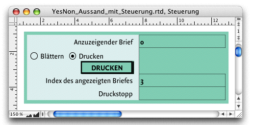
To scroll through mail merges, we need a control center on the one hand and a different formula structure in the address lines on the other. Let's take a look at the control center first. To do this, we create a «Control» spreadsheet, in which cell D4 contains the line number of the current address. Cell D1 shows the number of letters. Buttons in cells A3 and B3 can be used to scroll (when the «Browse» radio button is active). When the selection radio button «Print» is active the displayed letter can be printed. Our finished control center could look like Fig. 2.101 and Fig. 2.102.

Fig. 2.101:

Fig. 2.102:

Fig. 2.103:

Fig. 2.104:

Let's proceed step by step to set up the control center. In the two figures (Fig. 2.103 and Fig. 2.104), we have compiled the most important elements to provide a better overview of the functions. Let's first focus on the «Control» spreadsheet and leave the «Function» and «Print» buttons aside for now; they will be explained in more detail later. Since the formulas in the formula palette illustrations are easy to read, we will not repeat them in the text.

The formula in cell D1 refers to the “Function” button. This radio button with two options determines whether to «Browse» or «Print». If «Print» is selected (as shown in the illustration) then this cell should contain a 0. Printing is only possible if there is a «0» here – more on this later in the explanation of the «Print» button.

The formula in cell A3 is interesting in that it installs a «Back» button. However, this button should only appear if «Browse» («=1») is selected in the «Function» radio button; otherwise, this cell is empty. The button generated by the formula decreases the value in cell D1 by 1, but only as long as the value in cell D1 is greater than 1. Otherwise, the value remains unchanged.

Go directly to the next address

The formula in cell B3 is somewhat more complex. Here too, a button is first created («forward») – just as in cell A3. However, if certain conditions are met or not met, the «Print» button from cell F1 is placed in cell B3. If cell D1 is empty, the first address is displayed. With «forward», you should therefore scroll directly to the second address. Otherwise, the value in the cell is increased by 1 – but only as long as there is an entry in column B in the address table.

The formula in cell D4 displays the index from the address table. In «Browse» mode, the value from cell D1 is used. In «Print» mode, however, it is the print number. Both values are increased by «+2» so that the two header rows in the address table are skipped.

Unlike the «MailMerge» function, where RagTime detects when all addresses have been processed, the «PrintCycle» function cannot detect the end of the printing process on its own. Here, the «PrintStop» function must be used to specify where the printing process should be stopped. According to the formula in cell D5, the printing process should be terminated when an empty cell appears in column B of the address table.

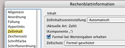
To prevent the formula from being deleted by manual entry in cells D1, D4, and D5, the cell or cell content must be protected. The easiest way to do this is to select cells D1:D5 and, under «Spreadsheet Information ➝ Cell Contents» check the box next to «Formula Preserved When Entering Values» (see Fig. 2.105)

Fig. 2.105:

Assign commands to buttons

In order for our control panel to be usable, we still need to add the commands or functions to the «Print» and «Function» buttons. We create the «Print» button in cell F1. We have designed this button specifically for this purpose, but the standard button generated by RagTime will also work. The design of buttons is described in detail in the chapter “Formulas Part 2: Variety of buttons”. In any case, our button needs a restriction so that it is only available under certain conditions. Open «Button Information» (double-click while holding down the “/6 key). Under «Arrangement ➝ Availability» enter the formula «Control!$D$1=0» (see Fig. 2.106).

Fig. 2.106:

The title under «General» is «Print» or «Printing», but the command must be «Print…». This button can therefore be used to start printing but only if cell D1 contains the value 0 or is deleted. The radio button «Browse»/«Print» in the merged cells A3:B3 is simpler. Under «General ➝ Title» enter the two terms «Browse» and «Print» one below the other and select «Return Their Index». Our control panel is now complete.

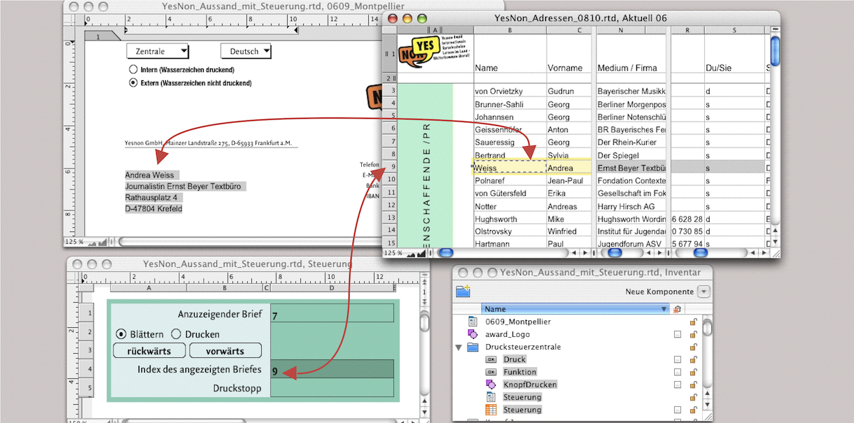
Only it cannot function as long as in the address field of our letter, it is still worked with the function «MailMerge». In this formula, «MailMerge» must be replaced by «Index». After the reference to the address spreadsheet or the respective column, «;Control!$D$4» must be appended. The entry for the entire address then looks like Formula 2.17, whereby we have also replaced the complete reference address of «YesNon_Addresses_0810.rtd» with «YesNon» to keep it shorter.

Formula 2.17:

Fig. 2.107:

Now you can browse with the “control panel” and review the letters individually before printing them. In addition, you can freely determine which letter you want to print individually. Since for larger mailings the address in the letter window is no longer sufficient, we turn directly to the topic of address labels.

2.5.8 «PrintCycle» for printing labels, too

If letters and enclosures do not fit into a standard window envelope when sending out mail merges the addresses must also be printed on adhesive labels. Since the mail merge function always prints as many copies as there are addresses, it is not suitable for printing sheets with consecutive labels, e.g. 30 per sheet.

In the following example, we assume that YesNon uses label sheets with 2 columns of 6 labels each, e.g. «Zweckform» labels No. 3659. Here, the individual label measures 97x42.3 mm. Depending on the label manufacturer, you may need to adjust the dimensions in the following example to suit your needs.

Setting up the layout

Open a new layout, delete the text frame, and create a new spreadsheet container of any size. You can also simply convert the existing text frame into a spreadsheet. In the «Object Coordinates» palette, enter all the information to adjust the size and position of the spreadsheet to suit your requirements (see also Fig. 2.108). Select six rows and four columns in the spreadsheet with the pointer and enter 42.3 mm for the height and 97 mm for the width in the «Object Coordinates» palette. For the sender on the labels, draw a new frame – you can also duplicate the existing frame – and give it the content type «Drawing».

Fig. 2.108:

See everything on the screen

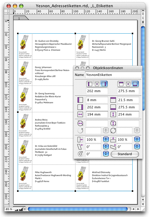
Open the drawing component and place the spreadsheet window and the drawing component window side by side on your screen, then open the Inventory and set it up so that you can see everything (see Fig. 2.109). Now import the logo for the labels into the drawing component and write the sender's address using graphic text. In the Inventory, give the drawing component the name «Sender», for example. Drag the drawing component from the Inventory to cell A1. Now, while working in the drawing component on a larger scale, you can see at any time how much space the sender needs on the label. When you are fine with the design, reduce the width of column A as necessary. Make a note of this column width.

Fig. 2.109:

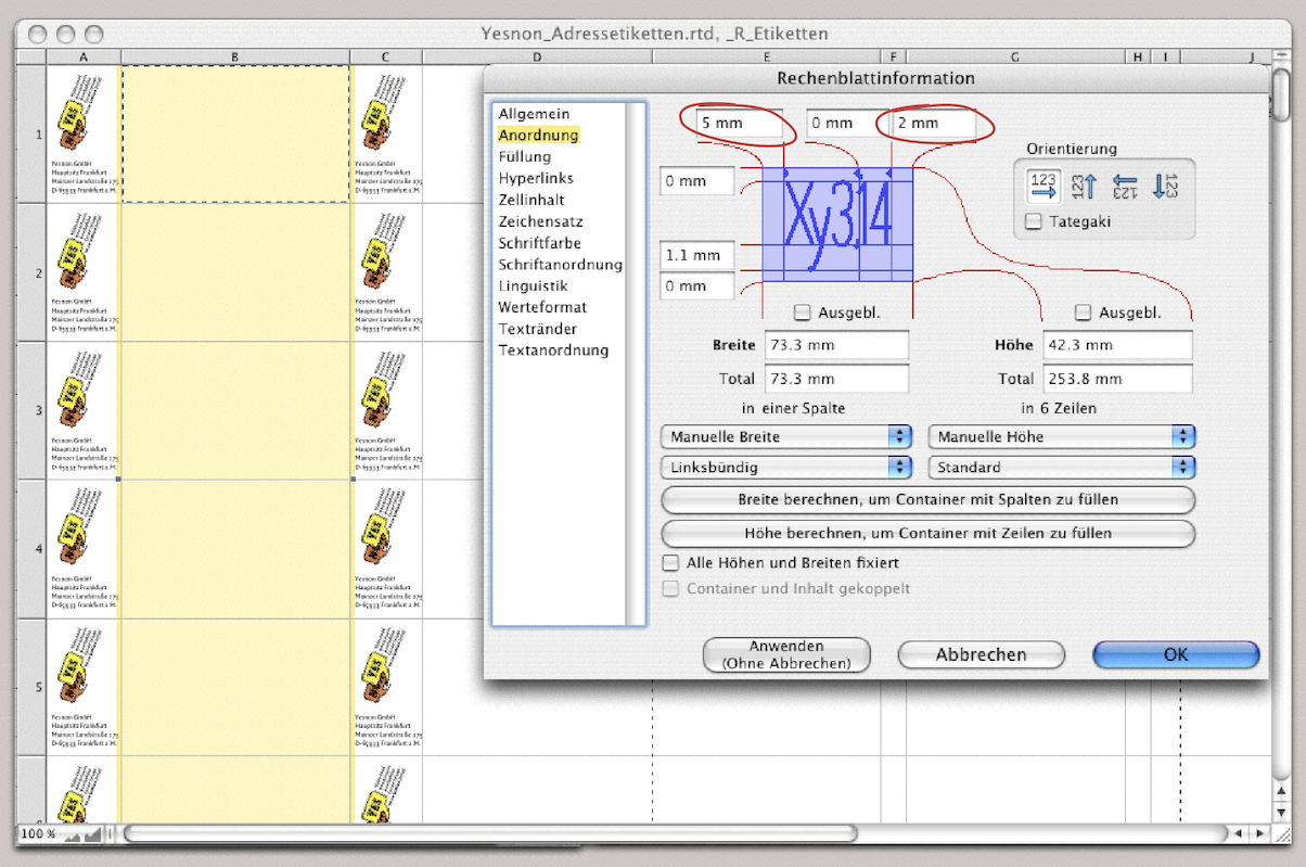
Fig. 2.109 shows the cumulative result of the following steps. The two columns together no longer have the desired label width of 97 mm. Work with an enlarged display scale, e.g., 150%. Select the two columns and open «Spreadsheet Information ➝ Arrangement». Under «Width/Total», it will then say «in 2 Columns»; enter 97 mm in the input field. Close the spreadsheet information and drag, in the column header, the dividing line between the two columns that are still selected to the left until the running display matches the noted width for column A.

Now select column B and enter 5 mm for the left margin and at least 2 mm for the right margin in the spreadsheet information. This creates the left and right margins for the address lines. In order for our formulas to take effect here, it is necessary to assign the content type «Multiline Text» to the cells. Close the spreadsheet information. Copy columns A and B, select column C – or the dividing line before this column – and paste the clipboard there so that these columns have the same formatting. Delete the duplicate of the “Sender drawing” in cell C1. To ensure that the same sender is used on all labels, enter an absolute reference to cell A1 as a formula in cell A2 and copy this cell to the sender fields of all other labels. If you now change anything in the sender, the change will be made in all twelve labels at the same time. Incidentally, you can make such changes anywhere: in one of the spreadsheet cells or in the drawing component itself, the correction will always take effect simultaneously.

And again: enter formulas

Each address cell contains the address via a specific index, which is derived from the page number (PrintCycle), column, and row. This index is used multiple times in each address. It would not be very elegant to calculate it multiple times in the same cell. Let's use cells B11:B16 and D11:D16 for this, i.e., the light blue cells in our open spreadsheet (see Fig. 2.110).

Cell B11 should contain the index of the first address in the address table – in the first sheet, this is 3, so that the header row is omitted. With each printed sheet, this number must be increased by 12 (number of labels). The formula in cell B11 therefore corresponds to Formula 2.18.

The other cells can refer to this cell B11 using the formula: «B11+1» in cell D11 and «D11+2» in cell B12. If you copy these formulas down the columns, the corresponding cells should now contain the values 3 to 14 in sequence.

In cell B20, we insert the formula for the print stop (Formula 2.19). This formula stops printing as soon as the row referenced by B11 of the address table no longer contains an address. The formulas for the addresses in the spreadsheet cells are now similar to those of the last mail merge (compare Formula 2.17). Only the reference in the index function must be different. Here, reference must be made to the cell in which the corresponding address index was calculated.

Formula 2.18:

Formula 2.19:

Formula 2.20:

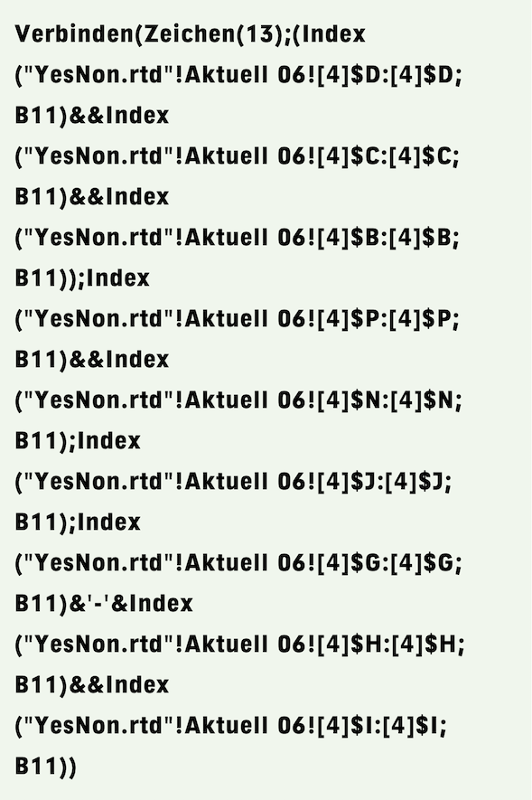
To ensure that the formula for the address only has to be written once and can then be copied into the other cells, we calculate the entire address again using a single formula (again abbreviated to «YesNon.rtd» for space reasons, where the complete reference address as in Formula 2.19 should actually be). This formula can now be transferred to all address cells by dragging and dropping.

Fig. 2.110:

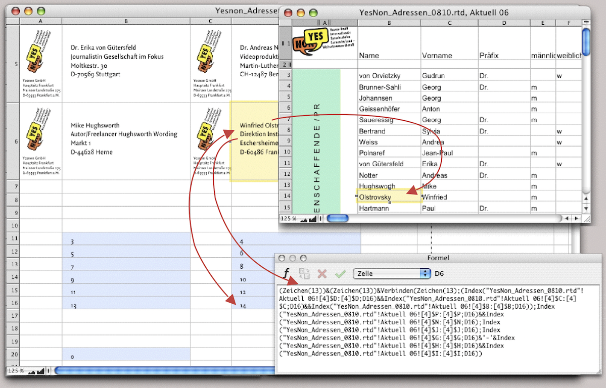
In the formula shown in Fig. 2.110, two blank lines are added at the beginning to position the address vertically in the cell. Fig. 2.110 also shows the formula in cell D6 and not Formula 2.20 in cell B3. It would have been possible to build the address line by line, as in the mail merge. To do this, the «Text in Cell» option would have had to be selected for each formula in the formula palette. However, this approach has a significant disadvantage! Relative addresses in such formulas are not automatically adjusted when copied to other cells. This would have meant that each formula would have had to be laboriously corrected. The somewhat larger and therefore less clear formula is preferable.

Finally, you can adjust the font style sheet for the address cells; an 11-point font is usually sufficient.

That's enough about mail merge, although there are still a number of special cases. If you have studied the above example, you now have the necessary tools to manage on your own.

Tips for mail merges

● Create formulas for mail merges whenever possible by dragging and dropping. ● Compile addresses for mail merges in text containers or multi-line cells in spreadsheets, not in multiple spreadsheet cells (with automatic content detection or text content). ● For labels, always use spreadsheets with multiline cells. ● Use «SmartConcat(Char(13);…)» to avoid empty lines in addresses and the double-AND operator «&&», to avoid gaps within lines. ● For browsing from letter to letter or for selective printing of individual letters, use the «PrintCycle» function instead of the mail merge function (do not forget the «PrintStop»). ● Compile the addresses in a spreadsheet in a separate document so that you can easily print the address list.

Fig. 2.111:

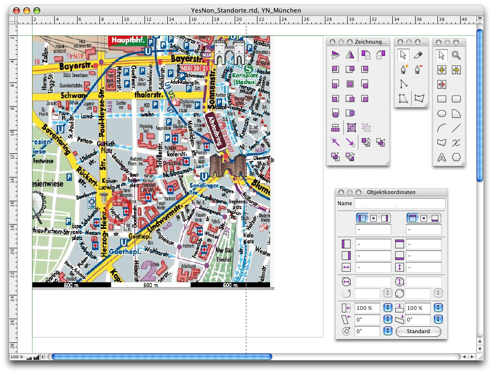
2.6 Drawing location maps

Our school has different locations; and the students should know where to find the respective YesNon school. Site plans, location maps, and access plans are essential for almost every company and event. Let's take the school in Munich as an example.

The classic approach is to obtain a template of the city map or the necessary section and draw over the desired parts. Those who work professionally with plans and geographical maps will probably use appropriate programs or extensions, or obtain maps from specialized providers (e.g. www.geoas.de)).

Planful setup

Get a suitable map section from the Internet or scan the desired city map. In this case, it does not matter which file format you use, as long as it is a format that RagTime “understands”. In our example, it is a PICT file (a screenshot of a web page). Open a new drawing component and drag the corresponding picture into this window. Pull the frame of the picture component a bit larger and fix the picture in the frame (double-click into the picture and set the checkmark under «Picture Information ➝ Arrangement» at «Fixed»). Then also fix the frame with double-clicking on it: «Drawing Information ➝ Objects ➝ Fixed». This ensures that the template is not moved while you are drawing.

Fig. 2.112:

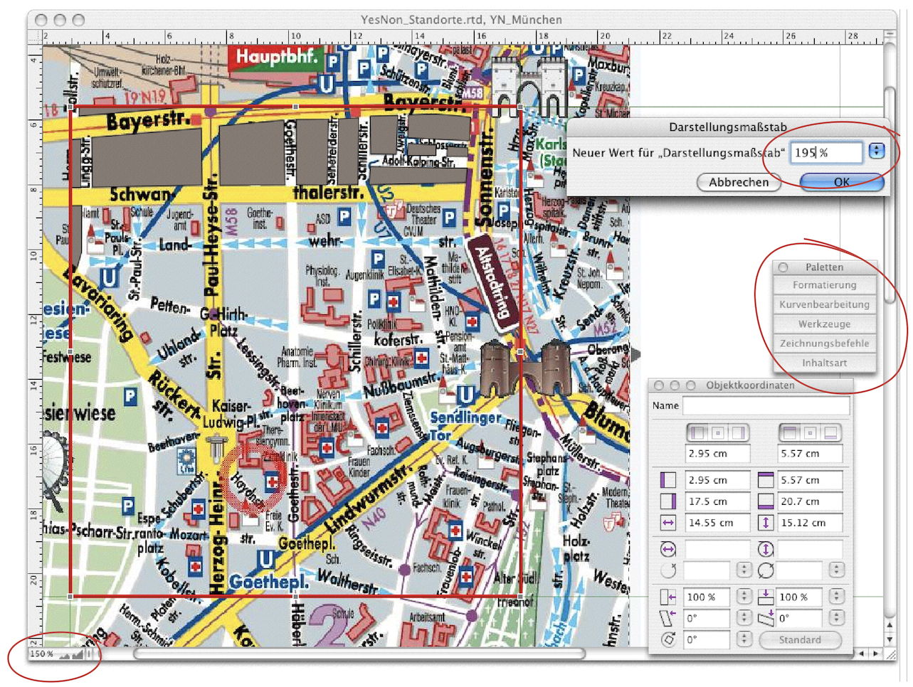
Save your document and then get the palettes important for drawing from «Windows ➝ Palettes» (see Fig. 2.111). As a reminder: if you are a Mac user do not need these palettes all the time and they are in your way, you can click on the green button in the palette header. This will bring up another palette, which is essentially a table of contents for the available palettes (see Fig. 2.112). If necessary, you can “click out” the temporarily hidden palettes again – they will then reappear where they were last placed on the screen. If you work a lot with drawings it is also worth creating some keyboard shortcuts here. Now you can of course immediately begin to trace the house blocks in polygons and Bézier curves. We have decided on a different workflow. We draw our polygons and elements for the location map in a second drawing component: pull a frame over the city map that should limit the map section. Assign the drawing component to this frame, assign it a transparent filling, and format the container border with a contrasting color. Then fix this frame so it cannot be moved. So now you draw your polygons and city map elements in a drawing component that is contained in a drawing component and lies above the city map template. This procedure is not unlike tracing with transparent paper. The advantage of this approach is that you can quickly switch layers while drawing and have all the objects you create immediately together in an independent component. You will need to switch layers frequently. It is therefore best to create two keyboard shortcuts here: one for «Drawing ➝ Stacking Order ➝ Bring to the Front» and one for «Drawing ➝ Stacking Order ➝ Send to the Back».

We have described the procedure in the section Define keyboard shortcuts. If you set, for example, the shortcut 1A“J/6“16 for «Bring to the Front» and 1A“H/6“17 for «Send to the Back» you can use the key combination to move a selected object forward or backward in a flash. See the “Keyboard Shortcuts Tables” in Appendix B “Keyboard shortcuts”.

What else you should keep in mind: you can “click through” a drawing component with a transparent frame, i.e., select objects behind it. The same applies to all transparent frames (rectangles, polygons, etc.). This behavior can sometimes be very irritating. If you want to click on objects in the drawing you have to work very precisely.

City planning: as large as desired

In addition to the magnifying glass and the magnification of the screen display via the icons in the lower left corner of the window, there is another size setting: «Windows ➝ Display Scale ➝ Other». Here, you can also enter completely individual scales. In the example shown in Fig. 2.112, 195% is of course quite special.

Now define a fill style sheet and, if necessary, line style sheets for all objects you will be drawing – buildings, green spaces, background (which counts as street color), parking garage and subway signs. Also define character style sheets for street names and the «P» for parking garage or «U» for subway. Now you are ready to start drawing the location map. If you are not yet familiar with the drawing component the following sections provide basic information, tips, and tricks. The Munich location map continues in chapter 2.6.8 “A few blocks away”.

Fig. 2.113:

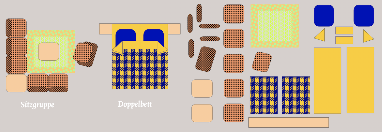
2.6.1 The drawing component

Of course, RagTime's drawing tools are no substitute for a full-fledged illustration program. But if you're less of an illustrator and more of a general-purpose user, RagTime offers a decent set of basic drawing tools.

Fig. 2.114:

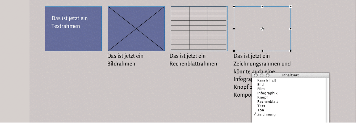
Quite apart from the fact that a drawing component represents a sophisticated “suitcase” in which, besides drawing elements, all possible other components can be packed, practically all basic drawings can be realized with Bézier curves, polygons, circle segments, and other predefined shapes. Here, too, the sophistication of RagTime becomes apparent: every closed line path – be it a geometric polygon or a free-form line – forms a frame that can also have content (any type of component) and thus becomes a container. Even open polygons and Bézier curves are closed with an imaginary line between the two endpoints and can thus become containers. This is why a rectangle, polygon, Bézier curve object, etc., which was created directly in the layout, is not displayed in the Inventory: because RagTime initially regards it as an empty frame or drawing object in the layout. Only when a component is assigned or corresponding content is imported is the corresponding symbol visible in the Inventory. At first glance, it seems contradictory that a drawing component can contain graphs, spreadsheets, or text and still be considered a «Drawing». Conversely, however, objects that look like drawings (as in Fig. 2.113) are simply a series of empty frames for RagTime (albeit with interesting, sometimes two-color fills and borders, they remain simple frames nonetheless). As mentioned above, only when a frame is assigned the content type «Drawing», regardless of its filling (see Fig. 2.114), RagTime lists this object in the Inventory as a drawing with the familiar ICON symbol. (Incidentally, the examples are taken from the document “Hausplaner” by Bernhard Storch on the expert pages of RagTime.de.) We have deliberately described this aspect in such detail because even experienced users sometimes forget this principle of RagTime.

Fig. 2.115:

Fig. 2.116:

Fig. 2.117:

Fig. 2.118:

Fig. 2.119:

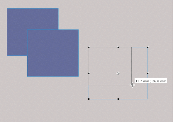
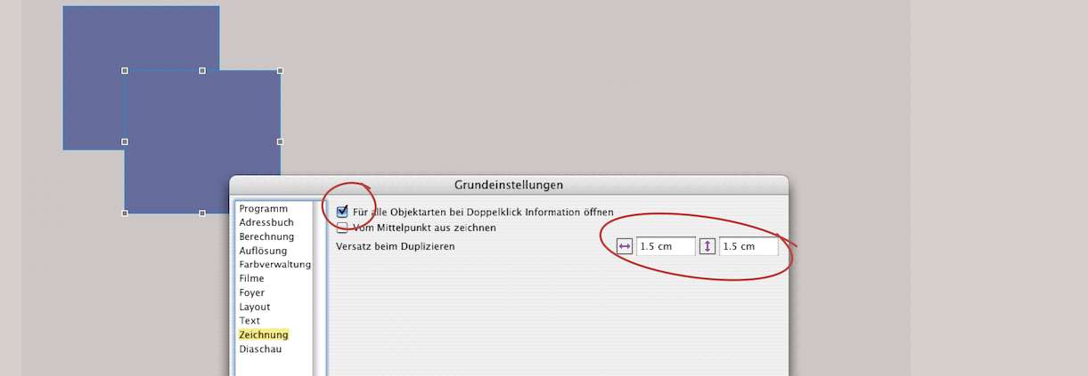
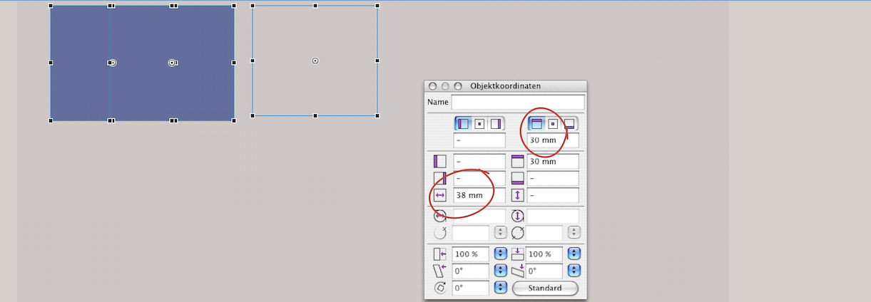
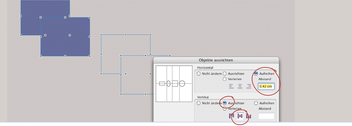
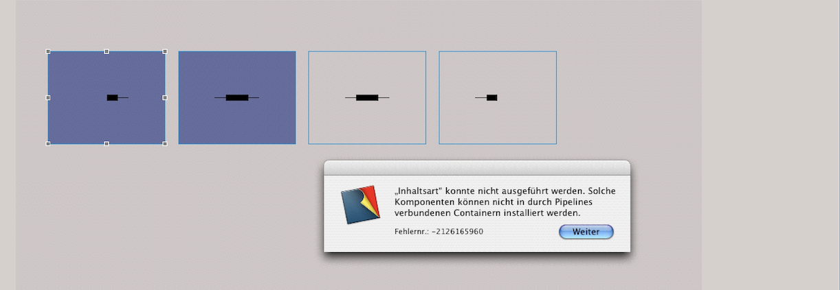
2.6.2 Not only for drawings

One of the advantages of RagTime's philosophy is that some functions and tools that are usually only needed for drawing can also be used for layout. One of these is, for example, the alignment of objects, accessible via «Drawing ➝ Arrange Objects». This function is extremely useful for creating text columns on the layout page and aligning various components. However, the above command only leads to the general alignment dialog. The drawing command palette, on the other hand, offers direct access to many alignment types. For an organizational chart or flowchart, for example, the commands «Align horizontally» or «Align vertically» are particularly useful, so it may be worthwhile to define a separate keyboard shortcut for these and other frequently used alignment commands (see appendix B “Keyboard shortcuts”).

Fig. 2.115 shows how the frames can be enlarged and reduced, with the current size of the frame always displayed in a display field next to the pointer. Fig. 2.116 is about the duplication of objects. Under «Extras ➝ Settings ➝ Drawing», you can define how far the duplicated object should be from the original object. Since this can be found under «Drawing», one might assume that this only applies to the drawing component. However, this function also applies to all objects. The input fields can also contain 0 or a negative value.

2.6.3 Object coordinates everywhere

The «Object Coordinates» palette is extremely useful. It can be used to “influence” almost all components, even spreadsheet cells or columns. You should always have this palette open in the palette dock, especially when drawing and layouting. In Fig. 2.117, for example, it is used to ensure that three different frames have the same width and all occupy the same position from the top edge.

2.6.4 Cleverly aligned

«Arrange Objects…» is a command that is logically only active when more than one object is selected. This opens the «Arrange Objects» window. In addition to the clear selection options «Centered», «Left», «Top», etc., each symbolized by three lines ICON , there are two other noteworthy options. In Fig. 2.118, all four objects are selected, and the setting command is: Align all objects vertically in the center and arrange them so that the distance between all objects is 12 pt (since «cm» was set in the measurement specifications, RagTime displays 0.42 cm here).

Tip:: A number of the palettes and functions used in drawing are generally useful for working with objects. Those who do not work with the drawing component very often may suddenly discover previously overlooked functions that will make their work much easier in the future.

The alignment of the objects will then look as shown in Fig. 2.119. Another setting option can also be useful, especially when layouting: suppose you have a defined type area and want to set your text in three columns. Draw a frame on the left edge of the type area, duplicate it twice, and move one of the copies to the right edge of the type area. Select all three objects and define the settings «Horizontal ➝ Distribute» and «Vertical ➝ Align ➝ ICON » in the «Arrange Objects» window. RagTime automatically sets the spacing between the columns. Of course, this is also possible with four or more objects and in the vertical direction as well. This allows you to quickly decide whether the column width and column spacing meet your expectations.

Fig. 2.120:

Fig. 2.121:

Fig. 2.122:

Fig. 2.123:

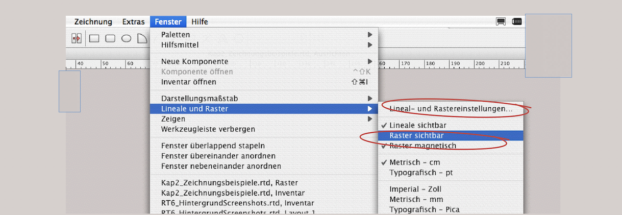
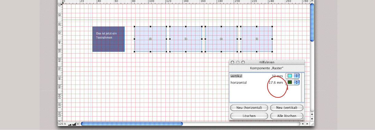
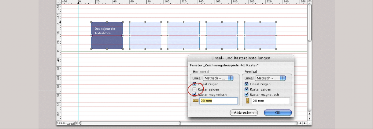
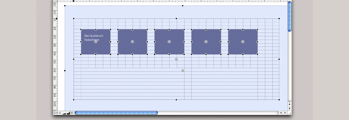
2.6.5 Pipelines and drawings

In Fig. 2.119, to demonstrate the pipeline functions, four frames without content were linked to a pipeline and then an attempt was made to define one of the frames as a drawing component. Of course, an error message appears: Drawing components cannot be connected to a pipeline. However, pipelines can lead away from and to components within the drawing component, which can also be very helpful for creative layouts. For example, you have a text frame in the layout and one, perhaps a picture caption, in the drawing component. Both text frames can be connected to a pipeline. The same applies to spreadsheet frames, of course.

2.6.6 Rulers and grid

Rulers and grids can also be used for all components. They are most useful when layouting and drawing. Under «Windows ➝ Show», rulers and grids can be set to visible/invisible, and the grid can be set to magnetic so that drawn objects already snap there at a small proximity to the grid line (see Fig. 2.120 and Fig. 2.121).

In Fig. 2.121, the «Guides» palette is open. Here, guides can be set vertically and horizontally in user-defined colors, independently of the grid: «Windows ➝ Palettes ➝ Guides». Guides can also be dragged individually from the displayed rulers into the active window – or back into the ruler to delete them. Double-clicking on a guide opens a small window in which you can select the exact position and color of the line.

Fig. 2.122 shows that RagTime treats horizontal and vertical gridlines separately. The «Rulers and Grid» window shown here can be opened with the menu command of the same name (circled in Fig. 2.120). In this window, you can also define whether only the vertical or only the horizontal gridlines should be magnetic. In addition, the zero point can be changed individually here. To adjust the grid spacing, you must select a different ruler from the pop-up menu, or even define a new one and then select it.

Grid also visible in the print?

Gridlines are understandably not displayed when printing. However, it is sometimes appropriate to work with permanently visible and printable grids. This is where one of RagTime's qualities comes into play again: the combination of different components. In Fig. 2.123, we have three layers: a spreadsheet in the background, which is set to the desired grid with the row heights and column widths.

Fig. 2.124:

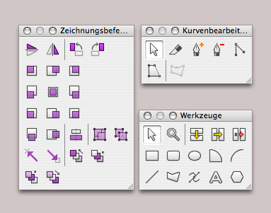
You must add printed lines to the cell borders. Place a large frame with no content over the top, which is given the fill style sheet «Transparent». In the illustration, we have given it a semi-transparent, light blue fill so that it is visible in the example. On the top, third plane, you can now create your drawings or set up text components. Depending on your needs, you can fix the individual containers or group them together.

2.6.7 Drawing utensils

Unlike in a traditional drawing program, the tools and aids for drawing in RagTime are not clearly arranged next to each other. Unfortunately, you have to search for them (see Fig. 2.124). Note the arrangement in the drawing command palette in the figure: only in this arrangement the nine alignment commands can be found quickly and intuitively, with the two for horizontal/vertical centering below them. This arrangement is achieved by changing the palette size. The most important object shapes, such as rectangle, rounded rectangle, oval, circle segment, arc segment, line, polygon, Bézier tool, and polygon, are all available in the toolbar in drawing and layout mode. The toolbar and other palettes can be brought up on the screen independently of the toolbar («Windows ➝ Palettes»). See also appendix A “Palettes”.

Fig. 2.125:

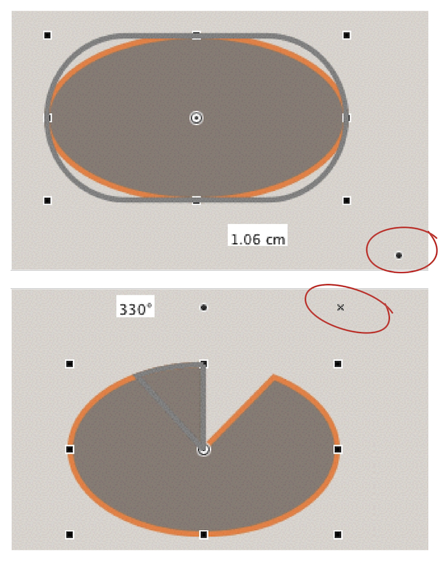
Almost all tools have additional special features: With the rectangle tool, you can draw squares by pressing the 1/1 key while drawing. With the ellipse tool, circles are created in the same way; for lines, a grid of 15° applies.

With the «Rounded Rectangle» tool, a point appears to the right below the drawing. If you click on it and move the pointer while holding down the mouse button, the radii of the object change. In the widest orientation, this can also create a rectangle again (see Fig. 2.125 top). A similar effect occurs with object types that were drawn with the sector or arc tool.

Sector or arc can be expanded or narrowed at a later point in time. In fact, every drawn object can be converted into another. A palette can be torn-off under «Drawing ➝ Object Kind» / click on the desired object type in this palette. Finished objects can be mirrored, tilted, aligned, grouped, ungrouped, and moved between layers using the «Drawing Commands» palette. (Fig. 2.124 left).

Take the tightest curves

The tools in the «Curve Editing» palette enable the following functions (from left to right):

Fig. 2.126:

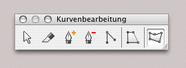
The pointer on the left helps you select and move drawn objects, lines, and anchor points. Depending on the object clicked, the pointer changes to a cross ICON or an ICON . The second tool, the «Curve Splitting Tool», can be applied directly to the line edge of polygons or objects drawn with Bézier curves (without having to select these objects first). If the lines of other objects are to be separated or “cut” they must first be converted. Unfortunately, the pointer in the form of the cutting knife moves without a position indicator. No positions are displayed in the «Object Coordinates» palette either. Cutting an object at two points results in two unclosed objects (see Fig. 2.128).

The two tools symbolized by a fountain pen have long names in RagTime. The pen with the plus sign is called the «Curve Point Insert Tool» It is used to set anchor points on lines that are equipped with tangent lines in order to draw Bézier curves (see Fig. 2.128, right circle). The pen with the minus sign is called the «Curve Point Removal Tool»; it deletes such anchor points.

Fig. 2.127:

Fig. 2.128:

Fig. 2.129:

Fig. 2.130:

Fig. 2.131:

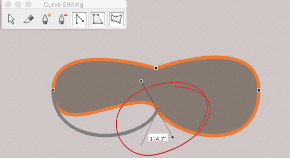
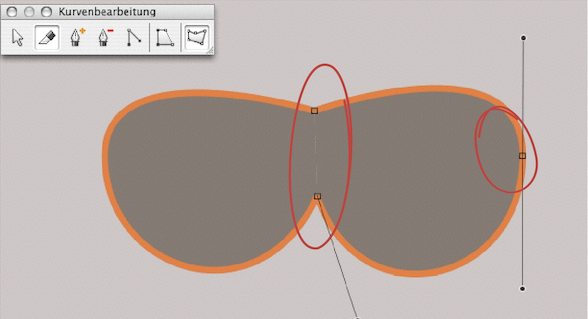
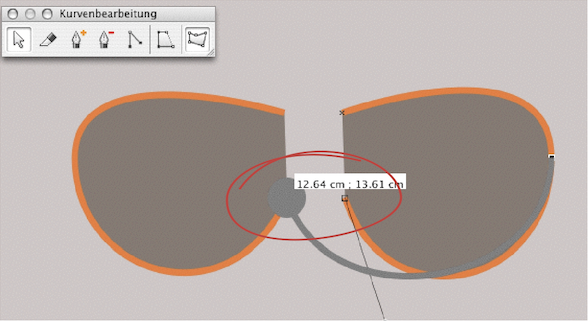
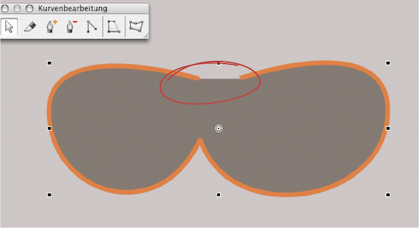
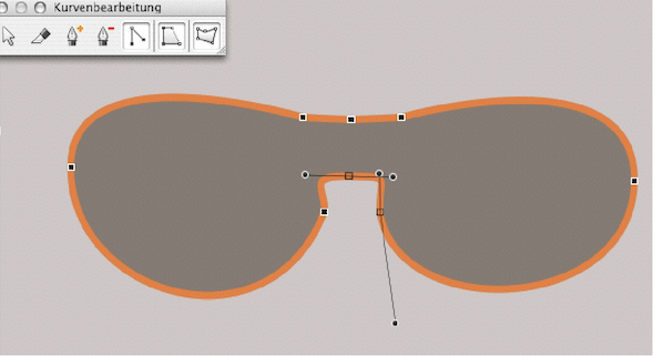
The «Curve Point Kink Tool» (5th from the left) transforms anchor points to allow a sharp angle in a polygon or Bézier curve object. This means that no anchor points are set, but existing ones are changed by placing the pointer at the end points of the tangent lines and moving it (see Fig. 2.127 and Fig. 2.131). If the pointer is placed at the Bézier anchor point, the tangent lines stretch back to an axis.

Fig. 2.132:

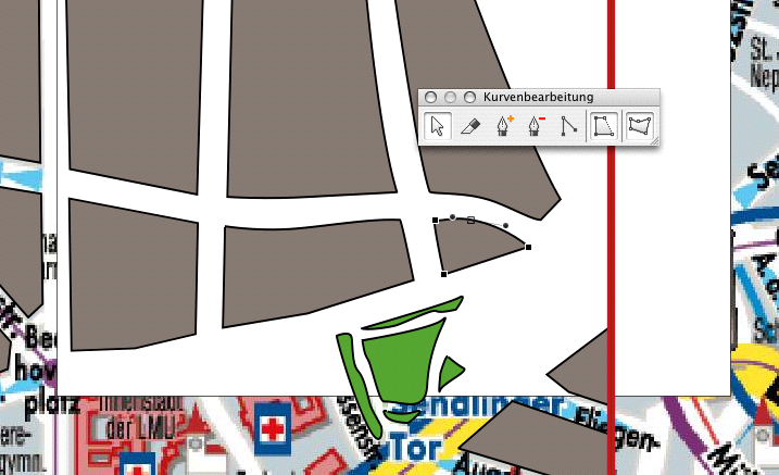
The sixth icon in the «Curve Editing» palette closes open drawing objects. Conversely, this tool can be used to reopen the last line segment of closed drawing objects (see Fig. 2.130).

Connecting drawing objects

Two drawing objects can be connected to each other if both objects are not closed. To do this, select the end point of one object and then move it to the end point of the other object while holding down the 3“/6“ keys. A thick dot with a small circle appears when the two ends meet (see Fig. 2.129). At the same time, the last drawing object moved takes on the line and fill style sheets of the drawing object just connected. If two different fill or line style sheets had been assigned in Fig. 2.129, the right object would take on the fill style sheet of the left object.

Important:: If content, i.e., a component (such as text), has been assigned to a drawing object, RagTime considers this object to be closed, even if the line border is still displayed as open. This object cannot then be connected. This can lead to confusion in the case of an empty text container, as at first glance it looks the same as a drawing object.

2.6.8 A few blocks away

In Chapter 2.6 “Drawing location maps”, we began drawing the Munich location map. Here in Fig. 2.132, we have already made some progress.

Fig. 2.133:

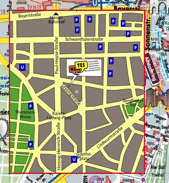
Since such a plan is not about all the details but about creating a good overall effect, the bitmap graphic behind it can sometimes be distracting. Here's a simple trick: insert a white sheet of paper between them. No, not literally, of course. But figuratively speaking, the effect is the same. We have the drawing component with the image of the city map, we have another transparent frame with a drawing component above it, and both are fixed.

If you now reduce the size of the window, you can draw a frame with white fill next to the upper drawing component, set it back one level, and then move it to the left until you can trace the details on the white background more easily (as in Fig. 2.132, the parallel course of the street curve).

Another little tip for working faster: to edit the lines of a Bézier curve or polygon object, you don't necessarily have to click on the «Edit Curve» ICON every time: With the object active, you can simply press the Enter key on the numeric keypad or double-click on a line of the object.

Signet and the color of the streets

Once all the blocks and green spaces have been drawn – don't forget to save your work regularly – we will add the nearest subway stations and parking garages to our location map. These can be text fields with blue fill, but also drawing components with graphic text.

The position indicator with the logo is a drawn polygon into which the logo has been dragged. The polygon thus automatically becomes a picture component. Now all we need to do in the drawing component with our blocks of houses and green spaces is to draw a rectangular frame over everything, which marks the streets and squares with the appropriate fill as a background. Of course, we also give this fill a style sheet so that we can quickly adjust the color scheme of the plan if necessary. The frame is moved to a lower layer («Drawing ➝ Stacking Order ➝ Send Backward»).

Labeling the location map

Use the «Text Tool» to write the most important street and square names and place them with a transparent background fill. Rotate them where necessary. The easiest way to do this is to grab the text object as a whole at its center point – the pointer will change to a rotation icon ICON – move the pointer slightly away from the center and then rotate. The outline of the rotated object and the current rotation angle are displayed (see Fig. 2.134). The «Object Coordinates» palette is used for fine-tuning the rotation angle and position: The input field at the bottom left is decisive for the angle (see Fig. 2.135). This procedure also applies to all other objects that you want to rotate.

Fig. 2.134:

Fig. 2.135:

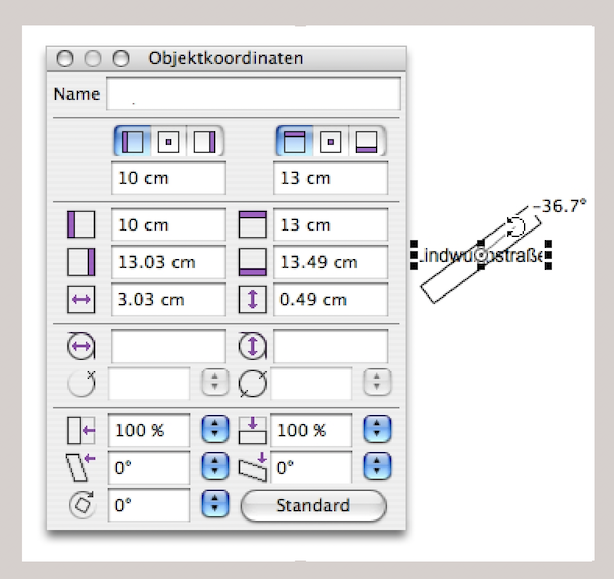
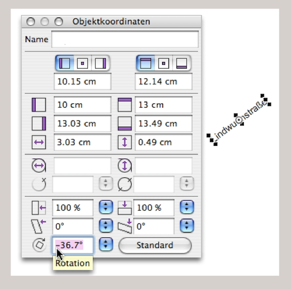
Our location map is ready. Since we have all the relevant elements in the same drawing component, we can drag them from the Inventory into a new layout or a new Inventory. The template with the city map can then be deleted. But be careful: don't delete it too soon. We had built our location map (as a complete drawing component) in a drawing component with the Munich city map template. If you delete the parent component – and the second drawing component in the Inventory had a check mark – it will also be deleted.

Rotating and shearing of the whole

If you have placed the location map component in a layout, you can also rotate and shear it (see Fig. 2.136), i.e., distort it into a perspective dimension (ideally using entries in the «Object Coordinates» palette). The interesting thing about this option is that text and all drawn objects are distorted in the same way. However, if you open the drawing component in its own window, you will find all objects in it exactly as you drew them. So it is not the objects that change, but the component as a whole. Incidentally, this works in exactly the same way as with image components, which you can also shear and rotate without changing the actual image.

Fig. 2.136:

Tips for working with drawings

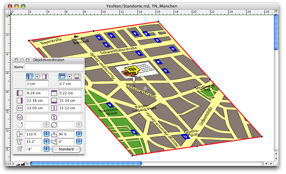
● If you often work on drawings with RagTime, assign keyboard shortcuts to all important drawing commands. This makes your work much easier. ● In particular, adjusting the display size («Keyboard Shortcuts ➝ Window Commands ➝ Display Scale») in two or three percent increments should be one of your shortcuts. ● In the formatting palette, under «Display», you can also adjust the size, even with differentiated input and quick switching to page or window size. ● With the magnifying glass, you can zoom in on a specific area of your layout or drawing. ● The palette dock is a useful tool on the Mac for keeping important palettes quickly accessible. ● Be sure to check out the settings for scales, guides (magnetic), and background grid (magnetic possible) so you can work with them. ● To make polygons and other drawn objects quickly editable: double-click the line or select the object and press the </T key. Pressing the </T key again selects the drawing object as a whole. If you need an object in the layout or drawing a second time, drag it to the desired location with the mouse button and “/6 key pressed. ● Use the option to convert object types, e.g., to turn a rounded rectangle or oval into a speech bubble: Convert to a polygon or Bézier curve, insert points, and insert the wedge. ● Use the option of working with several transparent or semi-transparent containers on top of each other to “trace” something. ● You can select an object behind it using an empty, transparent frame. ● This can also be confusing if you cannot reach the desired object: Check which objects have a transparent fill. ● Use the drawing component as a collection container to display different elements together. The drawing container can then also be used for the “image section” of the elements. ● Always work consistently with color, fill, line, and font style sheets when creating drawings.

2.7 And now it's the students' turn

That means planning! The basis for any planning is an agenda, a calendar. We plan for the long term and always want to maintain an overview, scrolling over the next year and a half. The agenda should always start at the beginning of the current week. To make the formulas easy to read, we only give short names to the frequently referenced components in our new «Planning» document. We make extensive use of the search functions in the following. If you are not yet familiar with them, please first take a look at the chapter “Formulas Part 3: In full swing”.

Fig. 2.137:

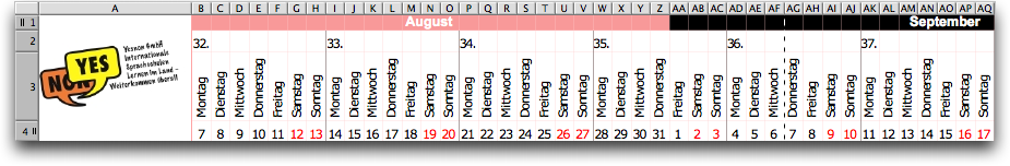
2.7.1 The calendar is scrollable

Our calendar needs a header that should look like the one in Fig. 2.137. The first four rows of the newly created «Agenda» spreadsheet are defined as title rows so that they appear at the top of each page when the planning calendar is printed. We place our logo in the united spreadsheet cells A2:A3. What is not visible, because we have set «Visibility: Nowhere» for this cell: cell A1 contains the date of the Monday of the current week. This date is determined using the following formula:

Formula 2.21:

Calendar with brains

To begin, we turn to the design of the calendar in the «Agenda» spreadsheet. The goal is to create a header as shown in Fig. 2.137. Row 1 contains the names of the months, alternating colors, row 2 contains the calendar week, row 3 contains the day of the week, and row 4 contains the date. In row 4, all days on which the school is closed should be displayed in red. These are all public holidays, including local ones, weekends, but also, for example, the week between Christmas and New Year.

First, we want to format the columns for one week. Select the 7 columns B:G and assign a line style sheet that you have created for this purpose to the right cell border using «Spreadsheet ➝ Borders… ➝ Right Border». Assign another line style sheet to the right border of column H. We have chosen a fine pink line and a fine black line (0.25 pt each). Thanks to the use of style sheets, you can change everything centrally if you – or the client – don't like the finished agenda.

Now select columns B:H. A quick tip: if you need to select a large number of columns and want to avoid tedious scrolling to the right, the easiest way to do this is to enter the desired range in the corresponding field in the toolbar (Fig. 2.138). Clicking on ICON accepts the entry as a range selection and opens the spreadsheet information at the same time. Don't be confused: the input field you just used now only shows the first cell (B1) of the selected range. However, a glance at the spreadsheet confirms that the selection was made correctly.

For the following dimensions, we assume the font «Arial» with a size of 10 pt, for which we have created a style sheet named «Calendar».

Fig. 2.138:

Fig. 2.139:

Fig. 2.140:

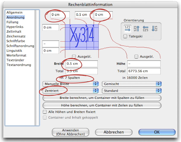
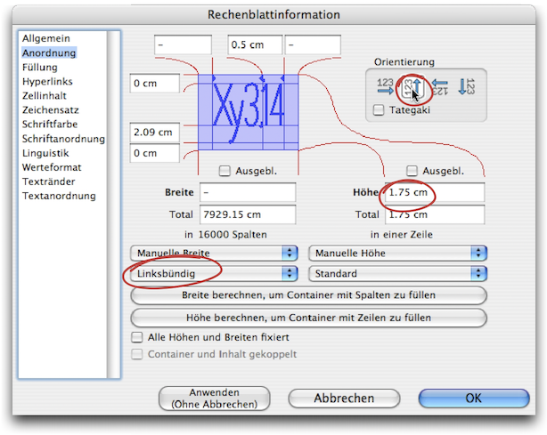
Check the number of selected columns in the «Arrangement» panel of the spreadsheet information (see Fig. 2.139). Set the column width to 0.5 cm, the distance from the cell margins on the left and right to 0, and the horizontal alignment to «Centered».

Close the info window and copy the area that is still selected with columns B:H. Select the first column to the right of this area and paste the columns there again. Do this as many times as you want weeks to be displayed in your calendar. Of course, once you have created the columns for 5 weeks, you can select all the corresponding columns and then add 5 weeks at a time using the same procedure. We did this until our calendar comprised 80 weeks = 560 columns. The last column of the calendar is then column UO.

Select row 3 and open the info window again (see Fig. 2.140), enter «Left Aligned» for the horizontal alignment, 1.75 cm for the row height, and select the second option for the «Orientation» with text running from bottom to top. While row 3 is still selected, assign it a value format of «Weekday», which is defined as «DDDD».

You need additional style sheets: a character style sheet «Month», e.g., inherited from «Calendar» but «Bold» and with the color «White». Assign the style sheet «Calendar» to the entire spreadsheet, then assign the «Month» style sheet to the first row. Create a fill style sheet «Month0» based on «Red Fill», but with only 40% density, and a second one, «Month1», inherited from «Black Fill», without changing anything. Of course, you can also choose other colors for these fills. The names are important because we will need them in formulas. To continue working, divide the window with the spreadsheet component «Agenda» so that you can see the first few columns on the left and the last few columns on the right of the area you just dimensioned.

Careful preparation pays off

Of course, we could enter a formula in each of the cells B1:B4 and copy it to the right as necessary. That would not be very elegant and unnecessarily inflates the document with all the formulas.

Fig. 2.141:

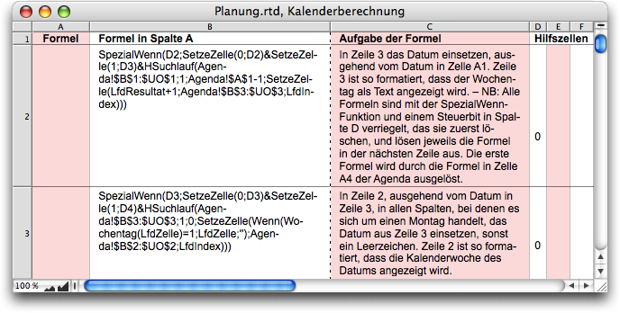
To improve clarity, we create a separate spreadsheet called «Calendar Calculation» for the formulas. However, this means that every reference to a cell or range in the «Agenda» spreadsheet is extended by the component name. It is obvious that we will need a whole series of searches, which we want to place in separate formulas. We use the technique of formula chaining with mutual triggering, which is discussed in detail in the formula chapter “Formulas Part 3: In full swing”.

In the «Calendar Calculation» spreadsheet, we use the columns as follows (see Fig. 2.141): the formulas are in column A. The value resulting from the execution of the formula is irrelevant and can only cause confusion. We therefore set the visibility of the cell contents for this column, apart from cell A1, to «nowhere» in the spreadsheet information. In cell B2, we insert a simple formula using the MetaFormula function «FormulaOf». This makes the formula in cell A2 visible in cell B2 (Formula 2.22).

Formula 2.22:

Please note: the displayed formula is only updated if the formula in the “monitored” cell results in a change in value. In «Spreadsheet Information ➝ Cell Contents ➝ Contents», specify that the formula should be retained when values are entered. This means that if the formula itself does not result in a change in value, you can simply enter a value in the cell after correcting the formula, and the formula display will be updated.

A word of warning: it is very tempting to make changes to the displayed formula rather than the actual formula. You should therefore definitely activate protection for the cells in column B – with «Extras ➝ Protection ➝ Formula Protected» and then «Extras ➝ Protection ➝ Lock Document» – preferably without a password. This makes more sense than simply preserving the formula when entering values, as was done earlier in column A. A formula changed in column B – it is only the display, not the actual formula – would not be checked for correct syntax when entered and would then have to be transferred to column A as the actual formula. – Of course, we copy cell B2 in column B down as far as necessary.

The reverse approach would also be possible: entering the formula as text and calculating it using the MetaFormula function «CalculateText». However, this would still lack syntax checking. If the input were syntactically incorrect, an error message would be displayed, but you would not receive any indication of where to look for the error.

To ensure that we can still understand each formula later on, we explain its function in column C. Additional comments can also be helpful. We will not provide more detailed documentation of the formulas here.

We use column D for mutual locking and triggering of the formulas: The formula in column A is only executed if the cell in columnD contains a 1. And first, the formula deletes this cell to ensure that the formula is only executed once. At the same time, the formula in the following row is released for execution. In columns E and F, the formulas store values that will be needed again later.

Now it should scroll

Formula 2.23 in cell A2 and other formulas can also be seen in Fig. 2.141 ff. However, there it is broken up in such a way that it is difficult to interpret. The first two lines of the formula show the lock with the value in cell D2, the deletion of this value, and the unlocking of the formula in the following row with the value 1 in cell D3.

Formula 2.23:

The formula part of the first two lines of Formula 2.23 is repeated in all subsequent formulas in analogous form. It is therefore only indicated here with «…».

This “standard part” is followed by the horizontal search, for which the range B1:UO1 is specified. This range is solely responsible for ensuring that the HSearch runs across all columns of our calendar. Which row of the spreadsheet is “searched” is completely irrelevant. The execution of the “follow-up value formula” is not subject to any conditions, hence the «1» as the “condition”. The starting value is the previous day (hence «-1») of the date in cell A1 of the «Agenda» spreadsheet. This date is therefore assigned to the value «CurrentResult» at the start of the HSearch execution. In each column traversed by the HSearch, «CurrentResult», i.e. the date, is first increased by one day and then inserted in row 3.

However, the date itself is not displayed there because we have assigned a «Weekday» value format to the cell. Nevertheless, the value of the cell is the date and not the text of the weekday. We use this in further formulas: In row 2, the week number should always be displayed on Monday.

The HSearch function in Formula 2.24 in cell A3 searches row 3 of all columns in the agenda and, if it is a Monday, transfers the date from row 3 to row 2. Otherwise, the cell is deleted. The row is assigned the value format «Date CW», which is defined concisely as «W». Once again, the cell may contain the date, but thanks to the assigned value format, it is displayed in a special way. There is therefore no need to supplement the formula with the function «WeekOfYearISO».

Formula 2.24:

For the next formula, which transfers the day to row 4, we need to do some more preparation. We want all days when the school is closed to be displayed in red. On the one hand, there is the useful function «ClWorkDayUSA», which recognizes working days in the United States. But even within a country, there are often additional regional holidays. In addition, there are days when our school is closed even though they are working days. And finally, we also have a school in Malta, but RagTime does not have a working day function for this country. The solution described below is universally applicable, i.e., it can also be used for Munich or Malta and the schools there.

Universal and regional holidays

We can find Maltese public holidays immediately by entering «Holiday Malta» into Google. We transfer these to a new spreadsheet called «Holidays». The table shown in Fig. 2.142 only contains these public holidays and would therefore need to be supplemented with the other days on which our school is closed.

Fig. 2.142:

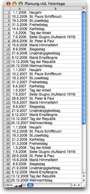
Whether you enter the holidays individually or derive them for the second and third years using formulas from the first is irrelevant here. However, we would like to provide the necessary formulas. Formula 2.25 for New Year's Day in cell A1 refers to the date in cell A1 of the agenda.

Formula 2.25:

This means that the holiday table automatically adjusts to the scrolling calendar each year. For holidays with a fixed date, such as «Independence Day» on July 4th, the formula for the first year is:

Formula 2.26:

The “New Year row” for the second year contains the Formula 2.27, which – thanks to the use of relative addressing – can be copied to all lines in the second and third years.

Formula 2.27:

A special case is, of course, Easter Sunday, which can swap places with Good Friday depending on the year. The calculation would always be correct, regardless of whether the days are in the correct or incorrect order in the table. Nevertheless, the incorrect order is unattractive and confusing. Formula 2.28 is entered in the row for the first of the two days and Formula 2.29 for the second.

Formula 2.28:

Formula 2.29:

The last two formulas can be copied into the corresponding rows for the following years, replacing the formulas used previously, as they also use relative addressing to refer to the beginning of the year. Add the days on which the school is otherwise closed to the table. You can leave a row in the table blank so that these days stand out clearly from the public holidays.

And now the formula that transfers these days to our calendar and displays them in red, together with the weekends. Once again, we use a value format – which we assign to row 4 in the «Agenda» spreadsheet – to influence the display. This time, however, it is not a matter of how the date is displayed. We use the option to automatically display negative numbers in red. We define the value format «Holidays» for this as in Formula 2.30.

Formula 2.30:

On holidays RagTime sees red

So we need to ensure that row 4 contains a negative number for all days that are to be displayed in red. This is done using Formula 2.31 in cell A4 of the «Calendar Calculation» spreadsheet (see also Fig. 2.143). The HSearch function searches row 3. The date found there is used to extract the day as a pure number using the «DayOf» function. The «If» function checks two conditions, which are linked with the «Or» function. If the day of the week is >5 it is a weekend day that should be displayed in red. The days that appear in the holiday table just created are also to be displayed in red.

Fig. 2.143:

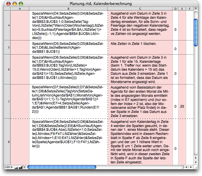
To determine this, the search function in the holiday table is used. These are nested searches in which the «CurrentCell» of the outer search – i.e., the HSearch across row 3 of the «Agenda» spreadsheet – is referenced with «CurrentCell(1)» and the checked cell of the inner search run – the one in column A of the holiday table – is simply referenced with «CurrentCell».

Formula 2.31:

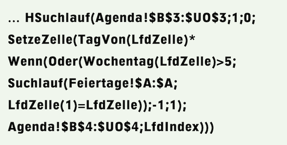
These two values are compared. If they match, the day is a holiday. There is a multiplication sign before the «If» function. The day determined by «DayOf» is multiplied by -1 or 1 depending on the result of the «If» check. The result is entered in row 4. To see that the formulas are actually working correctly, enter a 1 in cell D2 of the «Calendar Calculation» spreadsheet. The formulas are immediately executed one after the other, as we programmed them, and the “trigger” entered in cell D2 is deleted again immediately.

Formula 2.32 in cell A5 is trivial and requires no explanation.

Formula 2.32:

Deleting the entire month row beforehand simplifies the following formula, which only inserts the current date in the middle of the month and, thanks to the assigned value format «March», displays it as the month name. Let's allow ourselves a little “cosmetic luxury”: September requires the most space – 5 columns. If fewer than 5 days are displayed for the first month, we want to suppress this month name. And if it is displayed, it should appear in the middle of the displayed area. For the remaining months, we always display the month name on the 15th of the month.

Formula 2.33 in cell A6 processes all months except the first. Unlike the previous ones, this HSearch has a clear condition: the formula part for the subsequent value is only executed if the cell in question is the 15th of a month. However, whether the date from row 3 is transferred to row 1 also depends on whether the above condition is not met for the first time (CurrentCount>1) or whether the base day of the calendar is after the middle of the month (day of (Agenda!$A$1)>15).

Formula 2.33:

Formula 2.34:

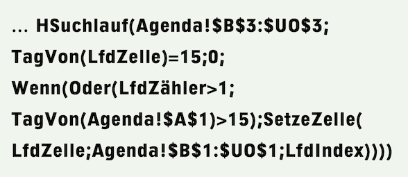
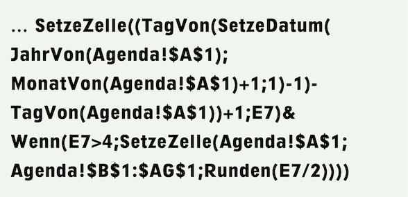
Then the first match that meets the search criteria is already in the second month displayed, whose name must be displayed in any case. Formula 2.34 in cell A7 basically consists of two parts and could therefore have been split again.

How many days does the month have?

First, the last day of the first month of the calendar is determined. This is done indirectly: First, the date of the first day of the following month is calculated using the SetCell function, and then one day is subtracted from it. The day of the base date of the calendar is then subtracted from this value, which is «31» if the first month of the calendar is August. This tells us how many days of this first month are visible in the calendar. This value is stored in cell E7 of the «Calendar Calculation» spreadsheet for later use.

The second part of the formula (starting with «If») first checks whether more than 4 days of the first month are displayed. If this condition is met the base date is inserted in row 1 of the agenda. Specifically, it is inserted in the column indexed by the rounded half of the value stored in cell E7 of «Calendar Calculation». This base date is always in the first month displayed. The fact that the data in rows 1 and 3 do not match is irrelevant, as only the month name is displayed. Now it is necessary to determine the first days of the month.

Formula 2.35:

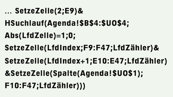
Formula 2.35 in cell A8 first stores the index of the first calendar column, i.e. 2, in cell E9 of the «Calendar Calculation». Starting with this row, the indexes of the first and last columns are stored in columns E and F for each month shown. To do this, the HSearch function searches for all first days of the month. For each hit, the «CurrentIndex» of the search corresponds to the index of the table column of the last day of the previous month. It is stored in column F. Note that the range specified in the second SetCell command only starts in row 10, i.e., one row further down. Therefore, the index of the column of the first day of the month is stored in the following row, column E. With each hit, the index to this auxiliary table increases by 1 thanks to the use of the hit count («CurrentCount»). Since the end of the last month displayed is outside the searched range, the last part of the formula, the third SetCell command, continuously enters the index for the last column of the calendar, i.e., column UO, in the following row of the auxiliary table.

Why is the end row 47 for the specified ranges in Formula 2.35? Pure coincidence! When creating the sample document, we probably specified row 50 as the end of the range, then deleted three lines, and the formulas were automatically adjusted. The main thing is that the specified range is at least as large as the table with the auxiliary cells.

Variable ranges, variable filling

The formulas in rows 9 to 28 of «Calendar Calculation» follow as a “dessert.” They are used to generate the different colors for the months in row 1. Each formula is responsible for coloring the columns specified in columns E and F of the auxiliary value table just created. The table has a small “catch”: depending on the base date of the calendar, one month more or less is visible in the calendar, meaning the table length is one row longer or shorter. The very last formula in cell A28 takes this into account (Fig. 2.145).

Couldn't all these formulas in rows 10 to 28 be replaced by a single formula controlled by a search? It's possible, but this construction would be so complicated that even experts might get confused. Sometimes it's necessary to assess whether the effort is worth the try. In this case, we decided against it.

Formula 2.36 applies to the first of these rows, row 9. It is formulated in such a way that it can be copied downwards. A prerequisite for this is the names of the two fill style sheets to be assigned. These names – «Month0» and «Month1» – differ only in the last character, 0 or 1. To determine the correct name for a variable range, there is the MetaFormula function «Range» to assign a fill style sheet to a range, and the Power Function «MPFSetRangeBknd».

Formula 2.36:

Fig. 2.144:

Fig. 2.145:

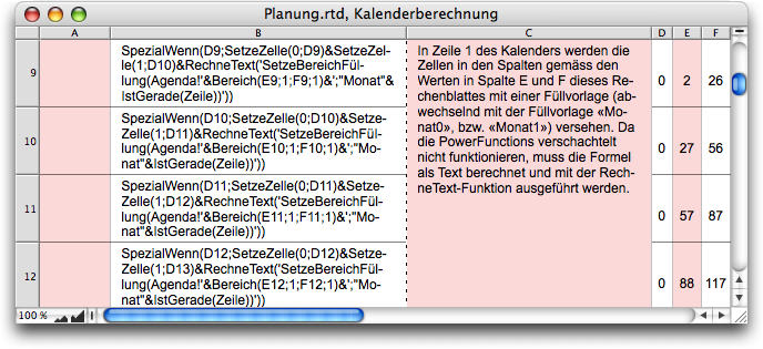
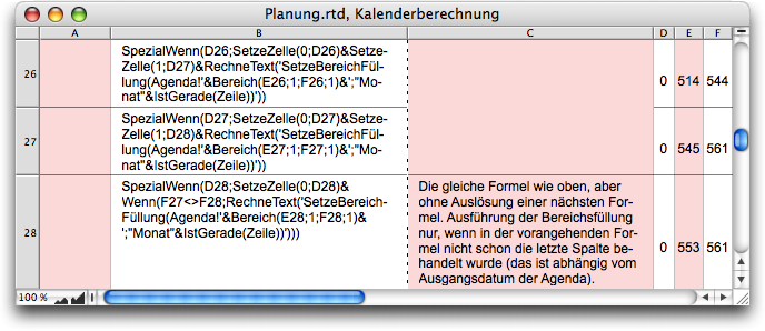
Please note: These functions cannot simply be nested. There is only one trick that works! We calculate the entire formula as text, in which the area to be filled is contained in the syntactically correct form. This text is then used as an argument in the MetaFormula function «CalculateText», which does exactly what its name suggests – it calculates the formula specified by the text exactly as if this text had been specified in the formula palette of the cell in question. The «CalculateText» function is always used when arguments of a formula, as in our case, must be calculated first.

It is also interesting to note how we achieved the variation in the fill. The function «IsEven(Row)» returns the value 0 or 1, depending on whether the formula is in an even or odd row. When calculating the text for the formula, this automatically alternates between the fill style sheets «Month0» and «Month1». Of course, we could have also worked with «Pink Filling» and «Black Filling». But then either every second formula would have been the same, or the formula would have had to assign the names of the two fill style sheets with an additional «If» function. The clever naming of the two fill style sheets simplified the problem.

Formula 2.37:

If you consider the case that arose in our example with the base date of August 7, 2006, you can see in Fig. 2.145 that the last two areas overlap, in accordance with the limits specified in rows 27 and 28. With this base date, one month less than the maximum possible is visible in our calendar. Therefore, no more filling can be assigned to the second of these two ranges. This is why Formula 2.37 looks slightly different from the previous ones. However, the first deviation has a different reason. It is the last formula in our sequence. This means that it does not need to trigger any subsequent formulas, and the second SetCell command is therefore missing in comparison to the previous formulas. However, the main part of the formula is only executed if the values specified in rows 27 and 28 in column F do not match. Either the operator «≠» or the combination «<>» can be used for «not equal». They are synonymous. The second option dates back to earlier times when many computers did not yet recognize the «≠» character, but is therefore often more familiar to experienced programmers.

Now all that's missing is the trigger for scrolling our calendar. We set the required formula in cell A4 of the agenda. Remember: thanks to Formula 2.21, cell A1 always contains the date of the Monday of the current week.

Formula 2.38:

At the beginning of next week, there will be a “larger” date there than in cell B3, where the displayed calendar begins. So now the calendar has to roll. It does this thanks to Formula 2.37.

As soon as such a date difference exists, the trigger for the first formula in our sequence is set in cell D2 of the «Calendar Calculation» spreadsheet. To test the formula sequence, you can simply enter a 1 in this “trigger cell” yourself. And off we go! There is so much to calculate that even fast computers need a moment! Please be patient! After a few seconds, everything is displayed as we intended.

Of course, there are many types of calendars that require completely different aspects to be taken into account. However, the above instructions can help you work out the solution yourself. In addition, there are the expert pages at RagTime.de, where you can find further solutions for calendars. You should check them out from time to time anyway.

And now it's time to plan

Our students' data is actually stored in the document with the addresses that we used earlier in this chapter. The formula chapter “Formulas Part 3: In full swing” explains how tables can be extracted, transferred, and sorted using RagTime. Your students could just as easily be recorded in a real database, i.e., with FileMaker or a database that has an ODBC interface. RagTime can then access the data with «FileTime» or «RagTime Connect».

Fig. 2.146:

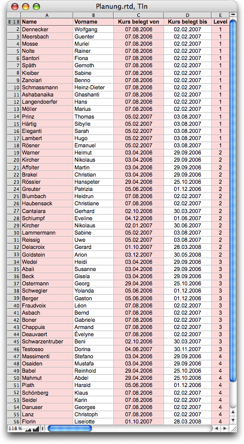
However, how you obtain the data is irrelevant for the planning we want to focus on here. So let's assume that the participant data is listed in the spreadsheet «Part» (short for «Participants») with the following information (see Fig. 2.146): in columns A and B, the last names and first names; in column C, the start date of the course; and in column D, the end date of the course. Finally, column E contains the course level. The table is sorted by course level («Level») and course start date. If a participant has booked two course modules, there will be two entries for them in the table.

Level 1 can only be taken twice a year on fixed dates for an entire semester. The other courses, on the other hand, can be started every week, as they are modular in structure. However, the duration of enrollment is constant, always six months. This does not make any difference to the following procedure, however. This circumstance must be taken into account when entering the participant data. Each course has a maximum of 12 participants.

In Malta, each course is only offered once. We therefore reserve 12 rows for each course in our planning agenda and give these blocks alternating background colors. To avoid color confusion, we use the same fill style sheets as in the calendar header. The empty calendar without occupancy or planning entries looks like the one in Fig. 2.147.

The names of the participants should be entered in this overview – if they are participating in a course that begins in the first week shown or has already begun, the name should be entered in column A. A bar, which still allows the calendar structure to be visible, should indicate the duration of the course. For all courses beginning later, the participant's name should appear at the beginning of the occupancy bar. The solution uses two different formulas for this. It would be possible to formulate these formulas in such a way that they cover all four course levels. However, we will refrain from doing so – the formulas are quite complicated anyway, as you will see in a moment. Here, we will only show and explain the formulas for the first course level in detail and indicate what needs to be changed in the formulas for the other levels.

Fig. 2.147:

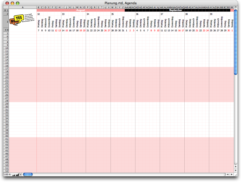
We use the same method as for calculating the calendar dates. The easiest way is to create a copy of the «Calendar Calculation» spreadsheet in the Inventory (simply drag it into the Inventory and hold down the “/6 key while dragging it a little) and name the duplicate «Occupancy Calculation». Of course, we delete the entries from row 2 in column A (formulas) and in columns C:F (comments and auxiliary values). However, we can leave the formulas in column B, which in turn make the formulas in column A visible. These formulas also always start with the lock function «SpecialIf» and the two SetCell commands, which delete the activation and trigger the following formula, again indicated only with «…» in the following formula representations. The first four formulas are shown. During formula creation, a test run can be triggered by setting the “trigger cell” to 1.

And now it continues as planned

In the first step, we want to develop a formula that searches for participants and enters them into the agenda; specifically, participants who are taking a course that has either already started or will start in the first week shown. The latter is the case in the example shown. However, with the right wording, these two cases can be handled together. As you may have guessed, and as you can now see in Fig. 2.148, the formula is not simple. But don't worry, we will go through it step by step. The first line of Formula 2.39 (see Formula 2.40) simply deletes the entire planning area, from row 5, the first row of level 1, to row 52, the last row of level 4, and from column A, with the name entries, to column UO, the last column of the scrolling calendar.

Fig. 2.148:

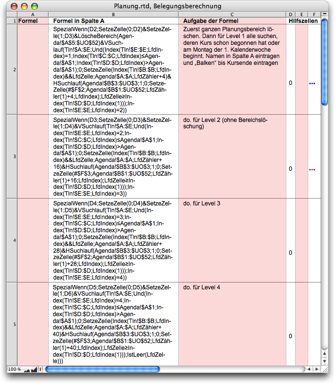
A vertical search then controls the whole process. Searched is the participant list «Part». Searched are those entries that correspond to several conditions at the same time, which are linked with «And» (see Formula 2.41). The first of the conditions is that only participants of level 1 are searched, thus rows with the value 1 in column E (see Formula 2.42). «CurrentIndex» always delivers the index to the just examined participant row.

A vertical search then controls the entire process. The participant list «Part» is searched. The entries that match several conditions linked with «And» are sought (see Formula 2.41). The first condition is that only participants from level 1 are searched for, i.e., rows with the value 1 in column E (see Formula 2.42). «CurrentIndex» always returns the index for the participant row currently being examined.

Formula 2.39:

Formula 2.40:

Formula 2.41:

Formula 2.42:

Formula 2.43:

Formula 2.44:

Please note that the table header is not explicitly skipped. This condition is certainly not met in the header.

The second search condition is that the course start date must be before or on the base date of the calendar, i.e., the value in column C must be less than or equal to this base date in cell A1 of the agenda (see Formula 2.43). Finally, course participants who have already completed their course should not be included – this is the third condition. Therefore, the end date in column D must be greater than the calendar base date. Hence Formula 2.44. This third condition is followed by the closing parenthesis of the «AND» function. The start value of the search is meaningless and is simply set to 0.

Now the name of the participant found should be entered in column A of our agenda, naturally on the first available row. This is done using a SetCell command.

Before we get to the name, we would like to point out here, as in the formula chapter “Formulas Part 3: In full swing”, that we deliberately avoid using the «ColumnValue» function. If, for example, we had used the seemingly simpler column value function (i.e., «ColumnValue(5)» for column E) in the condition according to Formula 2.42 instead of the somewhat complex index function, and then suddenly inserted another column into the table for some reason, our entire formula structure would have collapsed! RagTime cannot know that the absolute number «5» is actually meant to be relative, and it cannot automatically adjust it in the event of such a change. Have you ever tried to identify such an error and then find all the places that need to be corrected? We clearly prefer the index function, whose column reference is automatically adjusted if necessary.

We take the first name from column B and the last name from column A. Since column A is definitely the first column of the search range, we can use the «CurrentCell» function here instead of an index reference. We link the two parts of the name with the && operator, which automatically inserts a space (see Formula 2.45).

The name must, of course, be entered in column A of the «Agenda» spreadsheet, starting in row 5. Now, our search using the «CurrentCount» function always returns the number of participants already found, i.e., the value «1» for the first participant who meets all the conditions. With the addressing in Formula 2.46, the name is written in row 5 of column A for the first hit, in row 6 for the second hit, and so on.

And now for the bar!

Should we use the «MPFSetRangeBknd» command again, as we did for the month line when creating the calendar? That would be one option. But you may have noticed during testing that the construction with «CalculateText» and the variable areas seems to take a lot of computing time. And we'll soon discover a second reason why we prefer a different solution!

We opted for a pseudo bar, which is created by placing a character string in each day cell, which – when strung together – forms a kind of bar. To do this, we placed text in cells F2 and F3, one for a white background and the other for a pink background. The fact that we do not change the background but give the cells content helps us later to find out whether a particular date is already taken or not. The function part in Formula 2.47 helps us with this.

The “searched” area for the horizontal search, which is used to generate the bar, is actually meaningless. It is important that it starts in the first calendar column and runs far enough to the right. With UO, the last column of the calendar, we are far behind the end point of the bar to be generated, which will extend a maximum of six months from the start of the calendar. The execution of the follow-up value formula of the horizontal search is not subject to any conditions, hence the «1». The start value is also meaningless here.

Formula 2.45:

Formula 2.46:

Formula 2.47:

Formula 2.48:

Formula 2.49:

The SetCell command copies the aforementioned character string, including formatting (thanks to the «#»), from the auxiliary cell F2. The entire agenda for levels 1 to 4, i.e., from column B to column UO and up to row 52, is specified as the target range so that this part of the formula does not have to be changed when copying (see Formula 2.48).

The row in which the insertion must be made is determined by the outer vertical search. Because two searches are nested within each other, the «CurrentIndex» function must be supplemented with the “nesting level” (1). The column is determined by the running index of the horizontal search (see Formula 2.49).

Formula 2.50:

Formula 2.51:

Formula 2.52:

You may have noticed two things. First, the «+4» in Formula 2.49 would have been unnecessary if we had started the range in Formula 2.48 with B5 instead of B1. That's right! But when copying the formula for the other price levels, this makes it easier to find the place where adjustments need to be made. Second, we executed the SetCell function “unconditionally.” That's why we now need a termination condition for the horizontal search (Formula 2.50).

The search is terminated as soon as the date in row 3 of the calendar is equal to or greater than the end date specified for the participant in column D. Here, too, we must take the nesting level into account. And we see that it was correct to define row 3 as the search range for the search. Only in this way could we simply refer to the date in the column with «CurrentCell». The many parentheses at the end of this line close the nesting level of CurrentIndex, the index function, and the horizontal search.

We also need a termination criterion for the vertical search in the participant list (see Formula 2.51). Since this table is sorted by level, we can easily determine whether there is a level 2 participant in column E on the next row. Since we are no longer within the inner horizontal search, we can simply address it again with «CurrentIndex». Have we overlooked anything? To actually check the next row for this termination criterion, we would have had to write «CurrentIndex+1». That's right! Nevertheless, nothing wrong will happen because this row is still being processed. However, it fails the combined condition of the search and is therefore not processed.

You can copy these formulas down to level 2 for now. There, remove the MPFClearRange function at the very beginning. You can then copy this formula down further for levels 3 and 4. What do you need to adjust?

We refer here to the dissected subformulas, although the adjustments must of course be made in the formula as a whole. In comparison with Formula 2.42, the respective level must be used instead of «1». In the two formulas in which 4 was added to the sequential counter, Formula 2.46 and Formula 2.49, this value must be increased by 12 for each level. In Formula 2.48, adjust the reference to the character to be used for levels 2 and 4: row 3 instead of row 2, so that the character matches the background.

Finally, in the termination criterion of the outer search (Formula 2.51), levels 2 and 3 must be compared with the next level, i.e., 3 and 4. The corresponding formula for level 4 in cell A5 contains a different, much simpler termination criterion, as in Formula 2.52. Here, we no longer need to check the level in column E, but can simply see whether the next table row is empty, i.e., whether it no longer contains a name in column A. Since this is the first column of the search, «CurrentCell» is sufficient as a reference. In Formula 2.52, the three parentheses enclose the IsBlank condition, the vertical search, and the SpecialIf locking function.

Fig. 2.149:

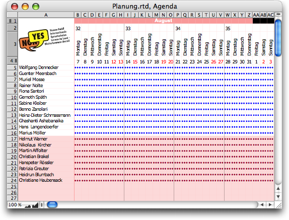
Our schedule is now looking quite neat (Fig. 2.149). However, it only gets really exciting in the later stages, where course registrations overlap at the higher levels.

Onward, as planned!

In the higher course modules, we can no longer simply insert a participant in the next row when there is a match, but must first find the first available row. Nevertheless, the structures of the formula just analyzed are repeated. Much of this will seem familiar to us. Here, too, we will only explain the formula for level 1 (Formula 2.53; Fig. 2.150) in detail.

The introductory commands are again only indicated here. The search range of the vertical search and the first of its three conditions correspond to Formula 2.41 and Formula 2.42. The second condition (Formula 2.54) requires that the course start date must be after the base date of the calendar, and the third (Formula 2.55) ensures that no courses are recorded that start after the planning period, i.e., whose start date is greater than the date in the last calendar column (see Formula 2.55).

Since the column with the course start date is needed several times, we store it in the auxiliary cell E6 using a SetCell command. This column index is calculated from the difference between the course start date and the base date of the calendar (calculated using the «AddDay» function) with a correction of 1 (see Formula 2.56).

Formula 2.53:

Formula 2.54:

Formula 2.55:

Formula 2.56:

Formula 2.57:

Formula 2.58:

Formula 2.59:

In this column, we then need to search for the first empty row in the level 1 courses area, i.e., a vertical search across rows 5 to 16 of the planning area (see Formula 2.57).

The cell in the column whose index we just stored in the auxiliary cell E6 must be empty. The «ColumnValue» function is suitable for formulating this condition (see Formula 2.58).

No, we didn't have to jump over our shadows to use this function. Here, we are not using it with an absolute column index, which can lead to errors when the table is changed, but with the index that we just determined and stored in cell E6, which is definitely correct.

We store the index of the first empty row found in auxiliary cell F6. Once the empty row has been found (1st hit), the search is terminated (see Formula 2.59).

At this crucial point, however, we want to pause briefly and take a look at why this row may be empty or contain something. If a participant is already scheduled for the course on the same row, we have created a “bar” with Formula 2.48 by writing characters in the cells for the duration of the course. However, there is a catch. For courses that do not coincide with the start of the calendar, the name of the course participant should appear at the beginning of the bar. We will insert this there with the next formula. However, in order for it to be displayed, the next cells must be empty. The next course participant cannot start until the following Monday at the earliest. So we just have to make sure that this cell is definitely occupied one week after the start of the course.

Fig. 2.150:

Formula 2.60:

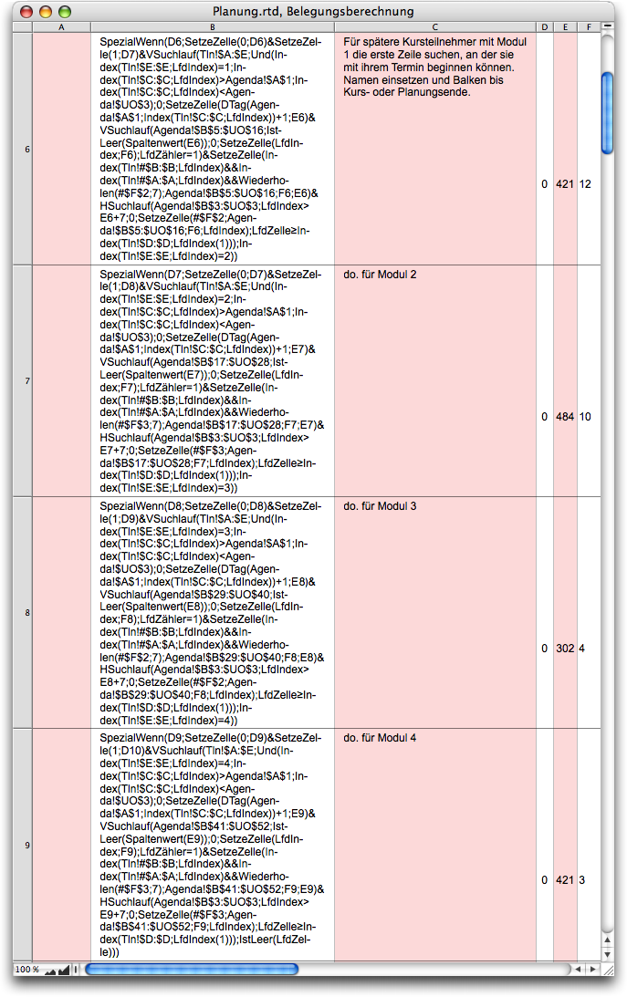
But first, let's insert the name. The first name is taken from the participant table as in Formula 2.45. Why can't we retrieve the last name using the «CurrentIndex» function as we did there?

This has to do with the rest of the value used! We add a space and seven hyphens to the name – with format transfer (see Formula 2.60). If the first name and last name are not also transferred with the format, the format of the “hyphen” dominates. And the «CurrentCell» function always returns an unformatted value. Even placing a «#» sign in front of it does not help. With the seven “bar characters”, we bridge the empty cells of the first week of the course even for short names – which have to be left empty so that the name can be displayed at all.

If you take a really critical look at the initial data, you will notice that a course participant is registered in level 4 with the course starting on January 2, 2007. However, this is not a Monday, but the Tuesday after New Year's Day. Perhaps by chance, another course participant in level 4 wants to start the following Monday. In this case, our planning would result in double occupancy of the course. So should we instruct our administration to always schedule the course start date on a Monday, even if that day is a public holiday? Hardly, because mistakes are bound to happen. Who would always think of such an instruction? We do not want to make the necessary adjustments in the main formula here, but only outline them:

Formula 2.61:

Formula 2.62:

Formula 2.63:

Formula 2.64:

The calculation of the column index to be stored in auxiliary cell E7 (Formula 2.56) must be corrected so that the column index of the preceding Monday is determined if the day on which the course begins is not a Monday. This is not that complicated. Instead of Formula 2.56, it should be Formula 2.61. Back to the name with the short bar that we still need to insert. The address is as in Formula 2.62. In other words, the calendar range for level 1 courses, indexed by the two values stored in helper cells E6 and F6.

As already explained, the next few cells must be left blank for the name to be displayed. However, to prevent the course from suddenly being booked again a week later, the following Monday must be occupied again with the “bar”. We take this into account in the condition that applies to the horizontal search that generates the bar. Apart from the condition in Formula 2.63, the search corresponds to that in the first group of formulas, Formula 2.47 and Formula 2.48, except that in the second of these formulas we have to limit the range to the rows of our price level (see Formula 2.64).

Fig. 2.151:

The termination criteria for the search runs are identical to those in the first formula group. The adjustments required for the other course modules in the copied formulas are similar to those in the first formula group. Find these necessary adjustments yourself – Fig. 2.151 can help you with this!

Planning moves along with the calendar

Finally, we need to ensure that not only the calendar rolls, but also the planning rolls with it. So, where there is a SetCell command in all the previous formulas to trigger the next formula, insert one in Formula 2.37 that sets cell D2 in the «Occupancy Calculation» spreadsheet to 1. This way, the end of the calendar recalculation also triggers a recalculation of the planning. If you have been successful, your planning in the rear area will now look like Fig. 2.147.

Did you break a sweat? So did your computer! On a MacBook Pro with a 1.83 GHz Intel Core Duo processor and 2 GB RAM, it took 35 seconds to calculate the calendar and planning with the participant data shown in Fig. 2.142.

Formulas: room for improvement!

Finally, a critical comment on the formula display in RagTime – certainly appropriate at the end of this formula-heavy section on calendars and planning: it would be very useful if the formulas in the RagTime formula palette could be wrapped, similar to what we have done here. And we have also been wishing for automatic multicolored brackets, always the same color for matching brackets, for a long time! On the positive side, we note the impressive performance of the functions and formulas. Anyone who works through a few exercises will be amazed again and again – but will also come up with ideas on how to solve problems more optimally.

RagTime Documentation Thomas Kaegi / Helmut Rodenhausen